helps you Microsoft Excel It organizes and analyzes extensive data using its spreadsheet software. It plays a vital role ranging from small to large-scale industries. Users can perform financial analysis with this powerful data organization tool. It offers a range of applications such as business analysis, people management, program management, strategic analysis, administrative purposes, process control, and performance reporting. However, it is primarily used for storing and sorting data for easy analysis. Microsoft Excel 2016 and 2019 support a feature where you can freeze a row or column in Excel. This way, when you scroll up or down, the frozen panes remain in the same place. This is useful when you have data spanning multiple rows and columns. Today, we will discuss how to freeze or unfreeze rows, columns, or panes in MS Excel.

How to Freeze/Unfreeze Rows or Columns in MS Excel
Excel's 1048576 rows and 16384 columns can store a large amount of data in an organized manner. Some other exciting features of Excel include:
- Data filtering,
- Data sorting,
- Find and replace feature,
- Built-in formulas
- pivot table,
- Password protection, and much more.
Additionally, you can freeze multiple rows or columns in Excel. You can freeze a portion of a worksheet row, column, or pane in Excel to keep it visible while you scroll through the rest of the worksheet. This is useful for examining data in other parts of your worksheet without losing headers or labels. Keep reading to learn how to freeze or unfreeze rows, columns, or panes in Excel. Microsoft Excel.
Important terms before you begin
- Freeze portions: Depending on the current selection, you can keep rows and columns visible while the rest of the worksheet scrolls up and down.
- Freeze top row: This feature is useful if you want to freeze only the first/top row. This option will keep the top row visible, allowing you to scroll through the rest of the worksheet.
- Freeze the first column: You can keep the first column visible while you scroll through the rest of the worksheet.
- Unfreeze parts: You can unlock all rows and columns to scroll through the entire worksheet.
Option 1: How to Freeze a Row in Excel
You can freeze a row in Excel or freeze multiple rows in Excel by following the steps below:
1. Press Windows key. Type and search in Excel and click to open it.
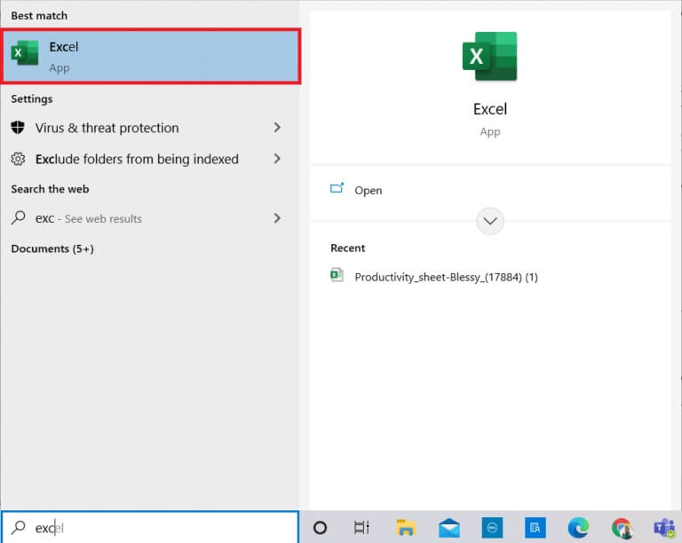
2. Open Excel sheet Required and specify any Row.
Note 1: Always select the row below the one you want to freeze. This means that if you want to freeze up to the third row, you must select the fourth row.
3. Then select "an offer" In the menu bar as shown.

4. Click Freeze panes > Freeze panes In the drop-down menu as shown below.
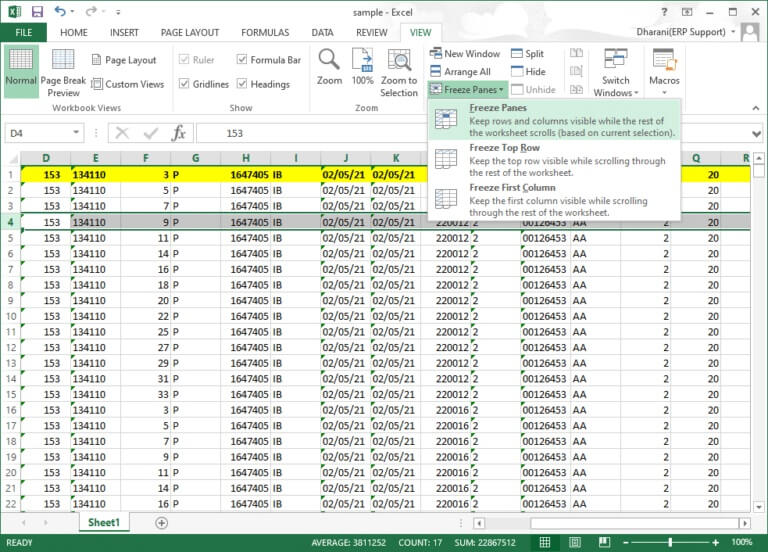
All rows below the selected row will be frozen. Rows above the selected cell/row will remain in the same place when you scroll down. Here in this example, when you scroll down, row 1, row 2, and row 3 will remain in the same place, and the rest of the worksheet scrolls will remain unchanged.
Option 2: How to Freeze the Top Row in Excel
You can freeze the header row in a worksheet by following the given steps:
1. Turn on Excel As before.
2. Open Excel sheet and select Any cell.
3. Switch to the tab "an offer" Above as shown.

4. Click Freeze Panes > Freeze Top Row As shown.
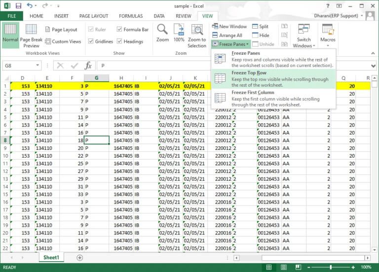
Now, the top first row will be frozen, and the rest of the worksheet will scroll normally.
Option 3: How to Freeze a Column in Excel
You can freeze multiple columns or a single column in Excel As follows:
1. Press Windows key. Write and search in Excel Click on it to open it.

2. Open Excel sheet and select Any column.
Note: Always select the column to the right of the column you want to freeze. This means that if you want to freeze column F, select column G, and so on.
3. Switch to the tab "an offer" As shown below.

4. Click Freeze parts and select an option Freeze parts As shown.

All columns to the left of the selected column will be frozen. When you scroll to the right, the rows to the left of the selected column will remain in the same place. Here in this example, when you scroll to the right, columns A, B, C, D, E, and F will remain in the same place, and the rest of the worksheet will scroll to the left or right.
Option 4: How to Freeze the First Column in Excel
You can freeze a column in Excel, i.e. freeze the first column in the worksheet, by following these steps.
1. Turn on Excel As before.
2. Open Excel sheet and select Any cell.
3. Switch to the tab "an offer" From above as shown.

4. Click Freeze portions This time, select the option Freeze the first column from the dropdown menu.
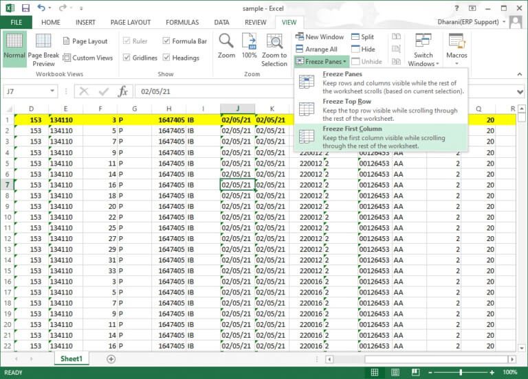
Thus, the first column will be frozen, and you can scroll through the rest of the worksheet normally.
Option 5: How to Freeze Panes in Excel
For example, if you're entering data into a report card containing student names and grades, it's important to always scroll to the title (which contains the subject names) and the label (including the student's name) frequently. In this scenario, freezing the row and column fields will help. Here's how to do the same:
1. Turn on Excel As before. Open Required worksheet and select Any cell.
Note 1: Always make sure to select a cell to the right of the column and below the row you want to freeze. For example, if you want to freeze the first row and first column, select the cell to the right of the first column and below the first row—that is, select cell B2.
2. Click on the tab عرض from the top bar.

3. Click Freeze parts As shown.

4. Select the option marked Freeze Panes as shown below.
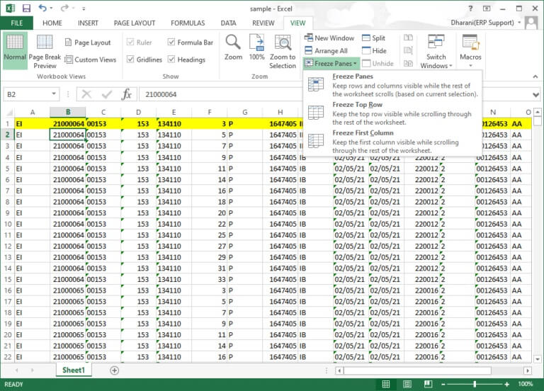
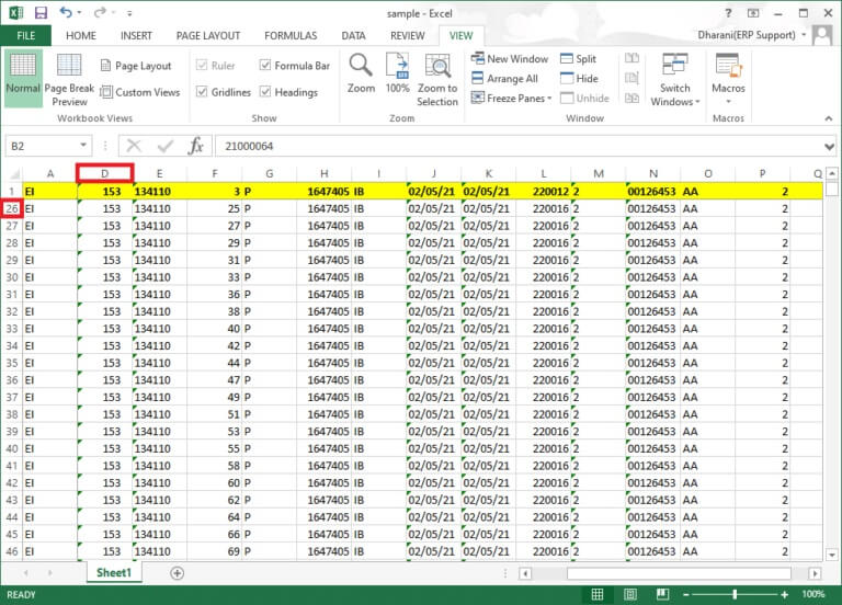
All rows above the selected row and all columns to the left of the selected column will be frozen, and the rest of the worksheets will be frozen. Here, in this example, the first row and first column are frozen, and the rest of the worksheet scrolls are frozen, as shown below.
How to Unfreeze Rows, Columns, or Panes in Excel
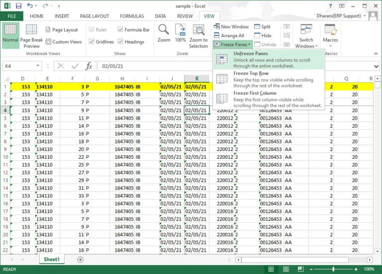
If you freeze any rows, columns, or panes, you cannot perform another freeze step unless they are unfrozen. To unfreeze rows, columns, or panes in Excel, perform the following steps:
1. Select any cell In the worksheet.
2. Go to the tab an offer.
3. Now, select Freeze parts And click “Unfreeze parts” As shown below.
Note: Make sure that no cell/row/column is frozen. Otherwise, the Unfreeze Panes option will not appear.
Pro Tip: How to Create a Magic Freeze Button
You can also create a magic freeze/unfreeze button in the Quick Access Toolbar to freeze a row, column, first column, row, or panes with one click.
1. Turn on Excel As before.
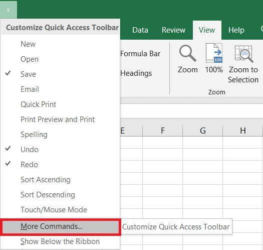
2. Click the down arrow, highlighted, at the top of the worksheet.
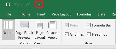
3. Click More commands As shown.
4. Select Freeze portions In the menu then click addition.
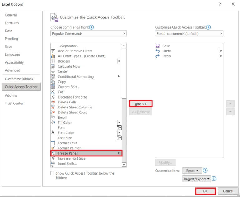
5. Finally, tap "OK". It will be an option Freeze Panes Quick Access Available at the top of the worksheet in MS Excel.
Frequently asked questions (FAQs)
Q1. Why is the Freeze Panes option grayed out in my worksheet?
answer. The Freeze Panes option turns gray when you're in edit mode or the worksheet is protected. To exit edit mode, press the Esc key.
Q2. How do I lock cells in Excel instead of freezing them?
answer. You can use the Split option in the View menu to split and lock cells. Alternatively, you can create a table by pressing Ctrl+T. Creating a table will lock the column header when you scroll down. Read our guide on how to lock or unlock cells in Excel.
We hope this guide was helpful, and you were able to freeze and unfreeze rows, columns, or panes in Excel. Please feel free to contact us with your questions and suggestions via the comments section below.


