There is hardly anyone who has not been faced with a situation of working on Microsoft ExcelOne could go on and on about the benefits of using this program. From small businesses to large enterprises, MS Excel has become a user-friendly application for everyone. Among its many functions, VLOOKUP is one of the most prominent, saving time for users with massive amounts of data. Can you perform a VLOOKUP with two criteria, or multiple criteria for that matter? Well, we've got you covered. In this article, you'll learn how to use VLOOKUP with multiple criteria using two methods, including using VLOOKUP with multiple criteria helper columns.

How to use VLOOKUP with multiple criteria
Continue reading to find the steps that explain how to use VLOOKUP with multiple criteria in detail with helpful illustrations for better understanding.
What is VLOOKUP in Excel?
VLOOKUP is short for Vertical Lookup. It's a built-in function in MS Excel that enables users to find specific values by searching them vertically across a sheet. This is done using a simple formula:
=VLOOKUP (lookup_value, table_array, col_index_number, [range_lookup])
here,
- lookup_value: This is the value you are looking for in the data.
- table_array: Specifies the location of the data where the desired values are located.
- col_index_number: Indicates the column number from which we will get the return values.
- range_lookup: It consists of two options. The first is TRUE, which indicates that you are looking for an approximate match. The second is FALSE, which indicates that you are looking for an exact match.
Can you do a VLOOKUP with two criteria?
Yes, you can perform a VLOOKUP with two or even more criteria. The VLOOKUP function can be used in two different ways using multiple criteria. One is a VLOOKUP with multiple criteria helper columns, and the other is a VLOOKUP with multiple criteria using the SELECT function. Read this article to learn more.
How to use VLOOKUP with multiple criteria?
Let's go over the methods you can use when wondering how to use VLOOKUP with multiple criteria.
Method 1: Using helper columns
It's one method you can use when you need to search for values based on multiple criteria. A VLOOKUP with multiple criteria helper columns requires you to follow the steps below.
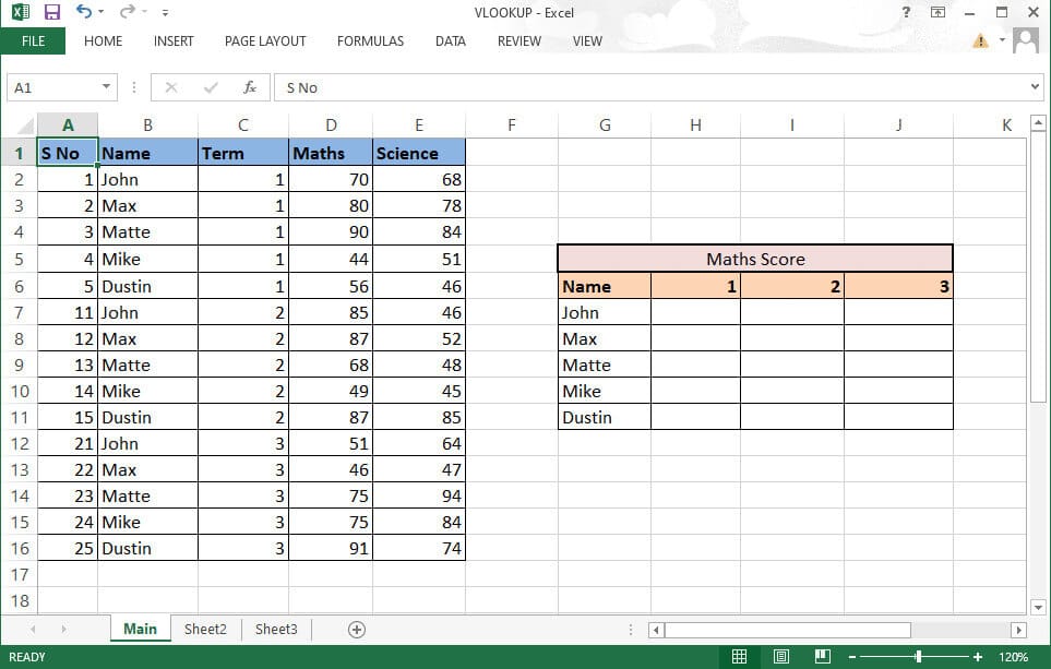
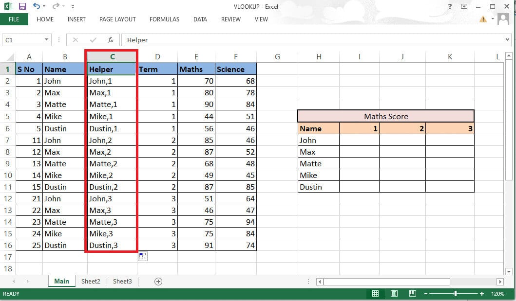
Note: In the steps below, we'll use students' math and science scores from grades 1, 2, and 3. The math scores across all grades are totaled. We'll find each grade's math score next to their names in the table on the right.
1. Open the file MS Excel With the required data.
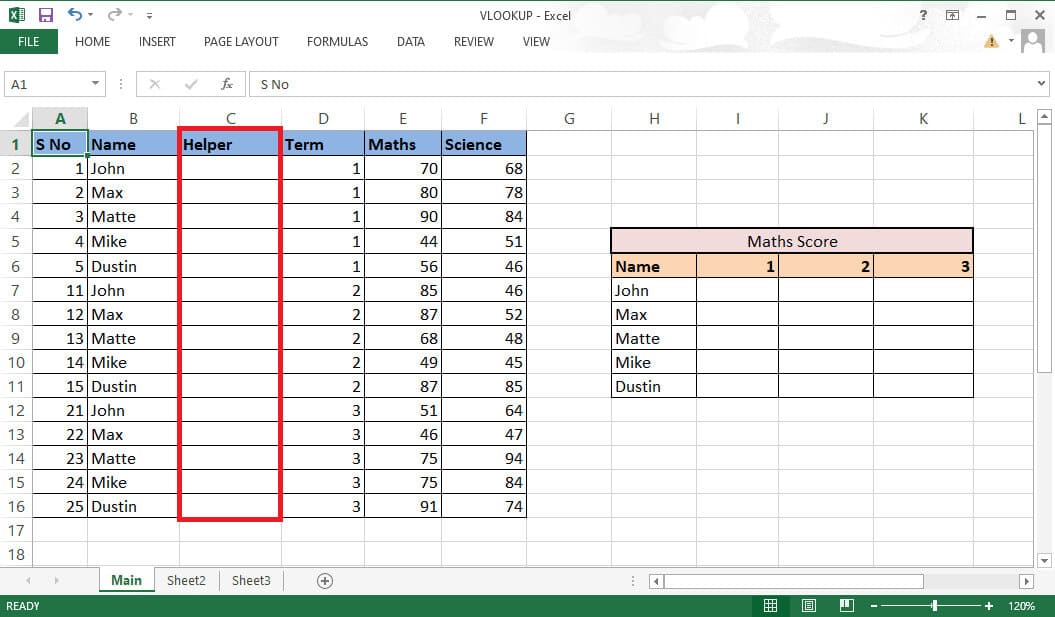
2. Enter New column Between the two columns you want to merge.
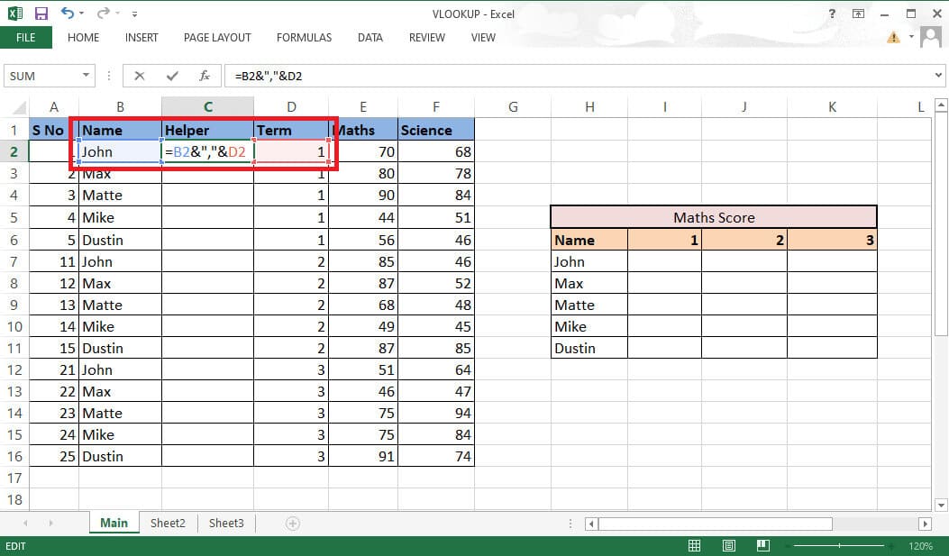
3. Collect Columns B and D using Ampersand (&) and comma (,) With the formula =B2&”,”&D2.
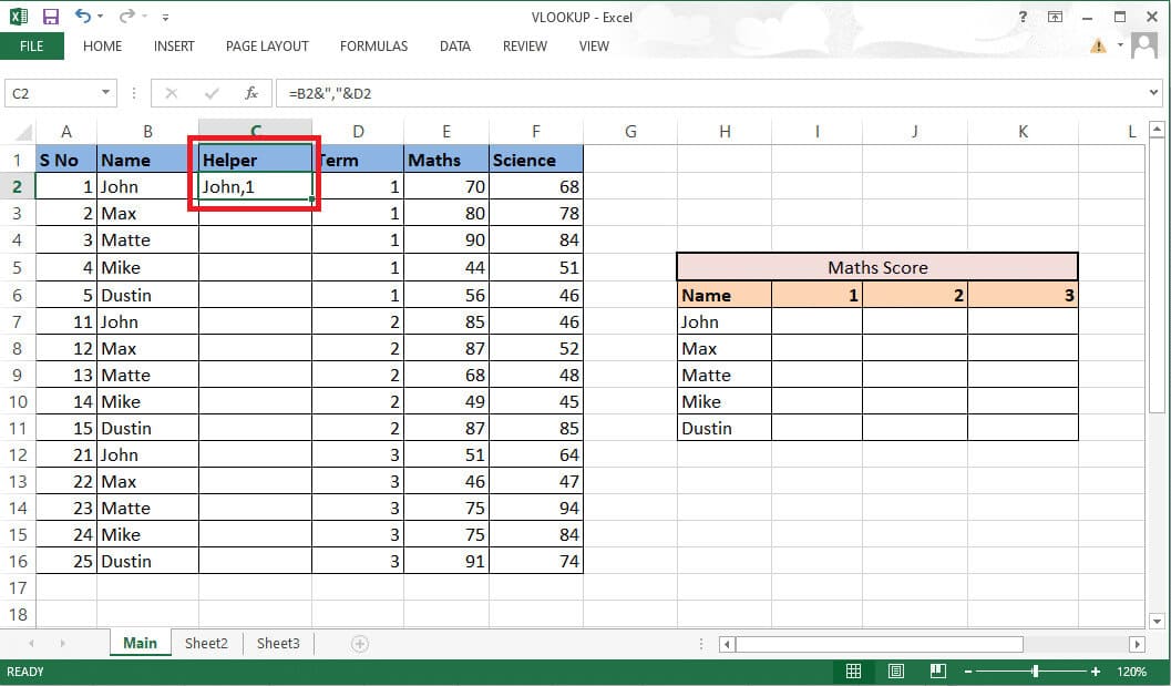
4. Press Enter key On the keyboard to see the combined result.
5. Pull formula To entire column To merge the remaining cells.
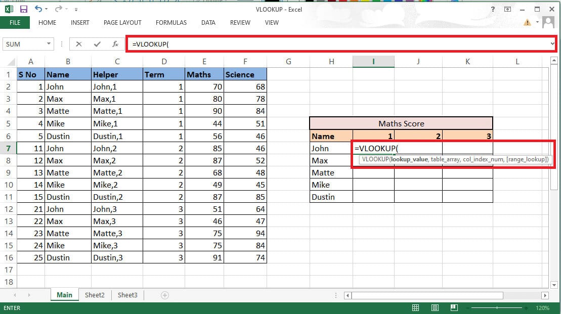
6. Enter VLOOKUP formula Where you want the grades. You can also view and edit the formula in the formula bar.
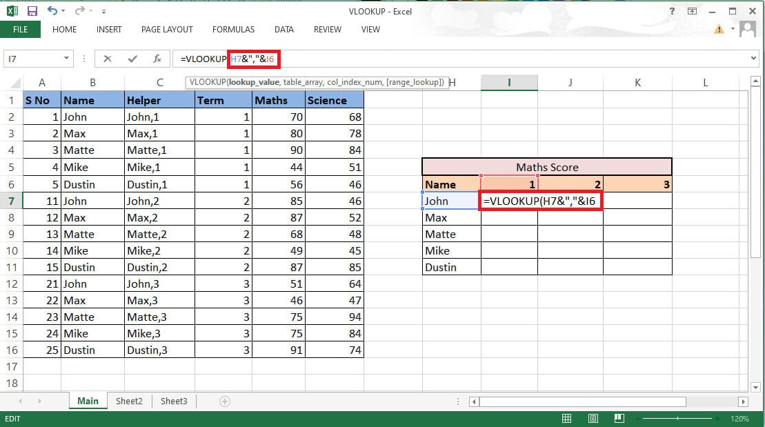
7. It will include: lookup_value cell H7 و I6 For reference. Write the formula as H7&”,”&I6.
8. Lock the rows and columns accordingly as we need to fill in the rest of the details as well. Lock Column H and grade 6 by pressing F4 . key To continue using VLOOKUP with multiple criteria.
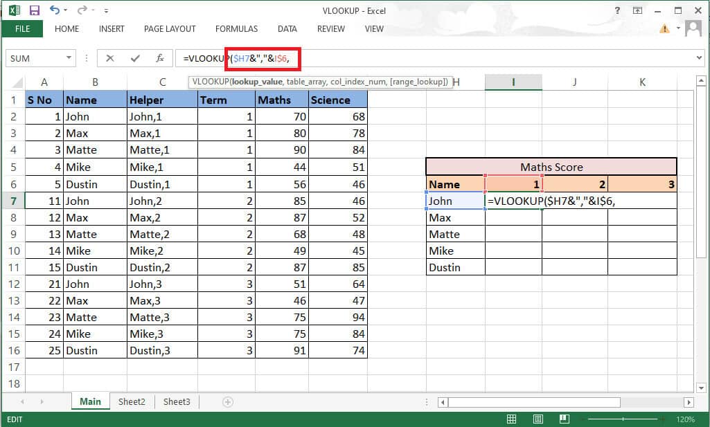
9. Go to the next parameter which is table_array By adding comma (،).
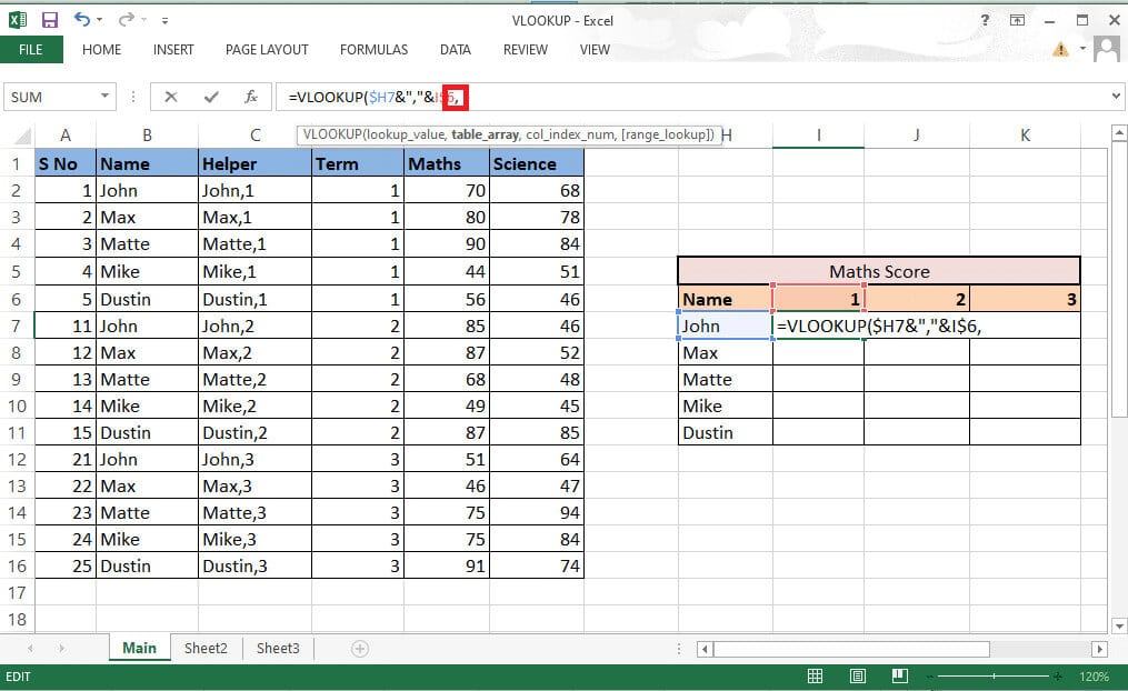
10. Select Rows and columns which contains Required values.
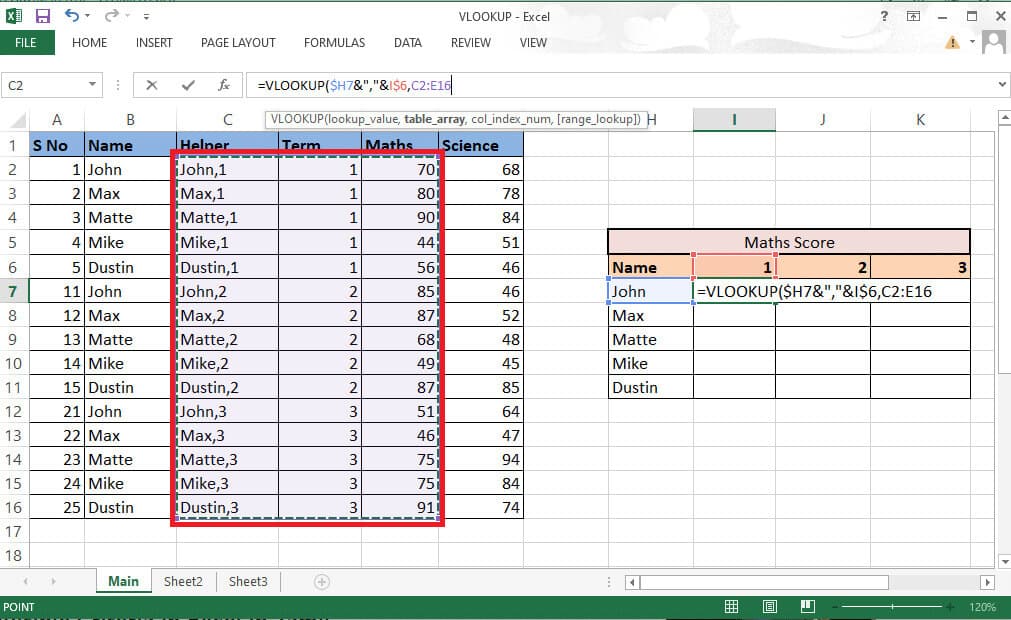
11. Lock the cell reference by pressing F4 key.
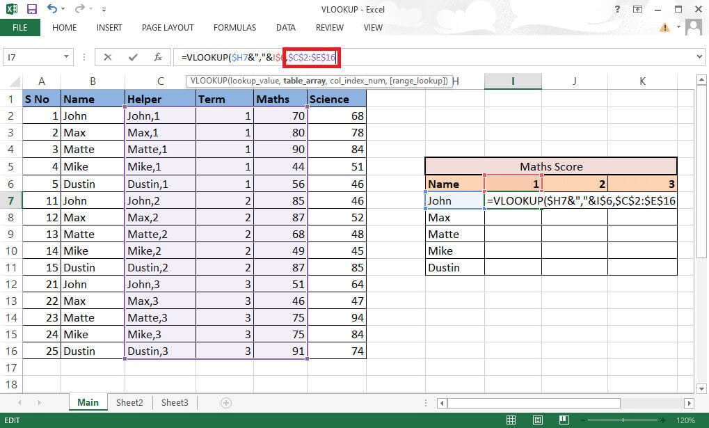
12. Add comma (،) Go to the next parameter: col_index_num.
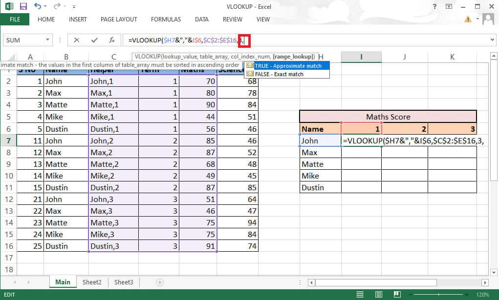
13. State the column number of the table array that produces the desired value. Here, the math column is the third. Write 3 In the formula bar.
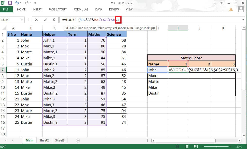
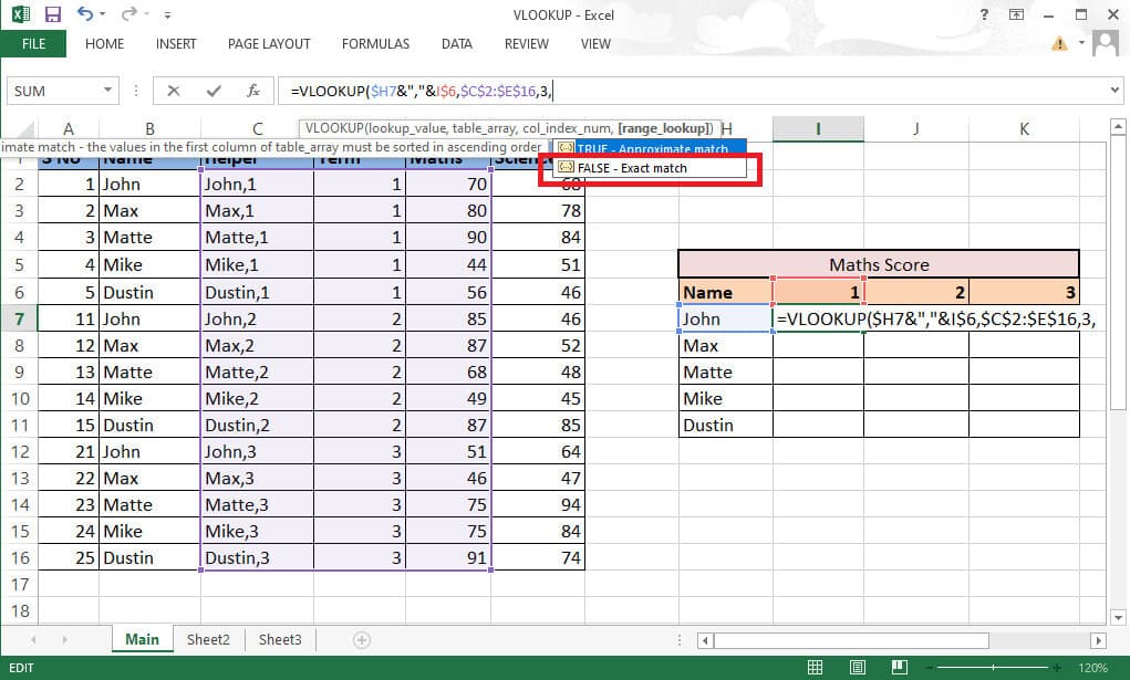
14. Write comma (،) To move to the next parameter range_lookup.

15. Select FALSE option – Exact match to follow to get the correct values.
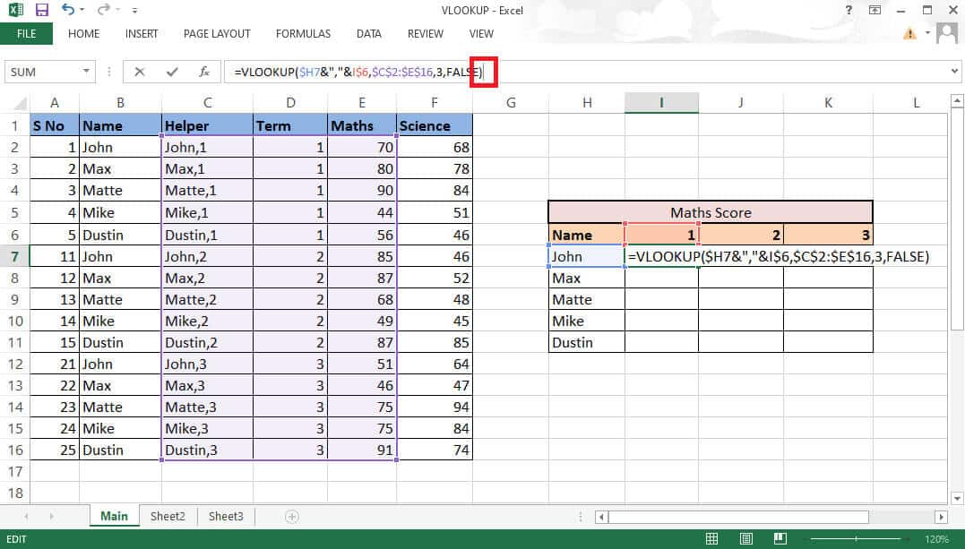
16. Close the bow After completing the formula.
17. Press Enter to get First value.
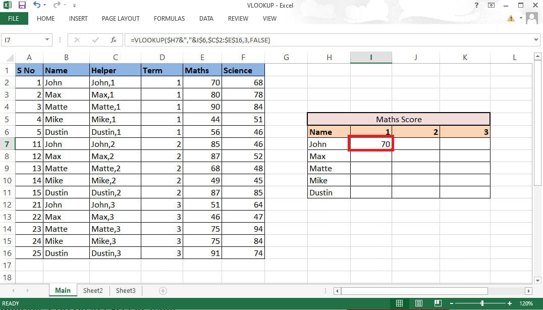
18. Drag the equation through the table to get all the required details.
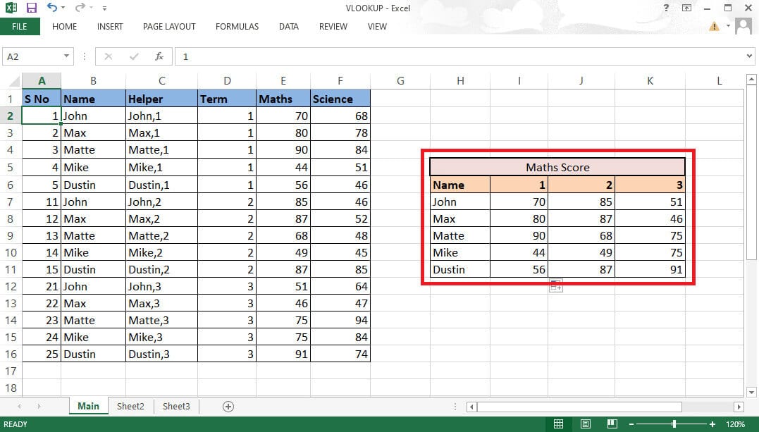
These steps should have cleared your doubts about the question, can you do a VLOOKUP with two criteria?
Method 2: Use the Select function
You can also include this method to use VLOOKUP with multiple criteria using the Select function. Unlike the method above, you don't need a helper column here. You can easily use the Select function option to use VLOOKUP with multiple criteria. Follow the steps below to use VLOOKUP with multiple criteria.
1. Go to File MS Excel With the required data.

2. Enter VLOOKUP formula In the required cell.
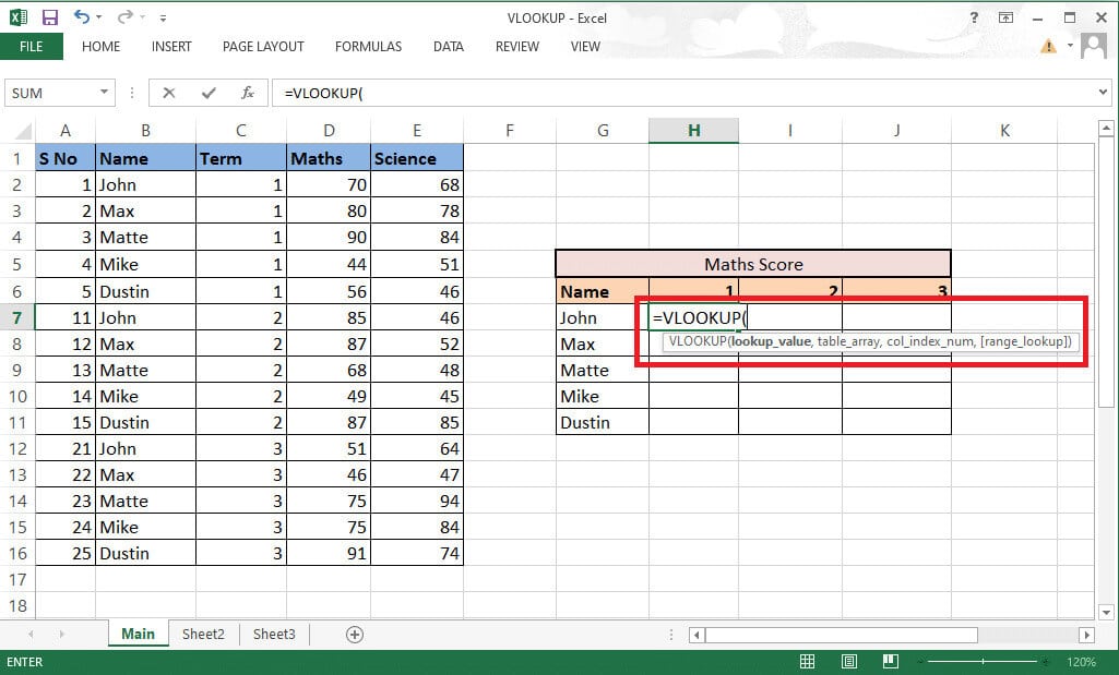
3. It will include: lookup_value cell G7 و H6 For reference. Write the formula as G7&”,”&H6.
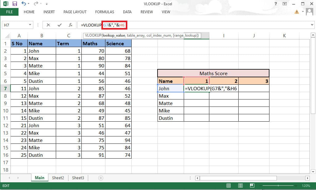
4. Lock the rows and columns accordingly as we need to fill in the rest of the details as well. Lock Column G and Row 6 by pressing F4 key.
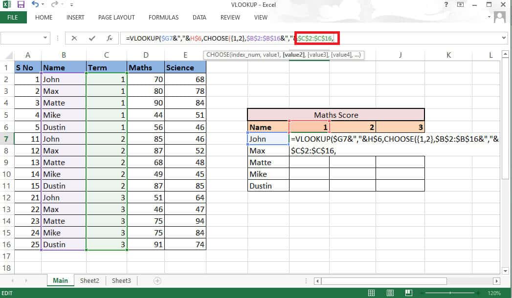
5. Write comma (،) To move to the next parameter.
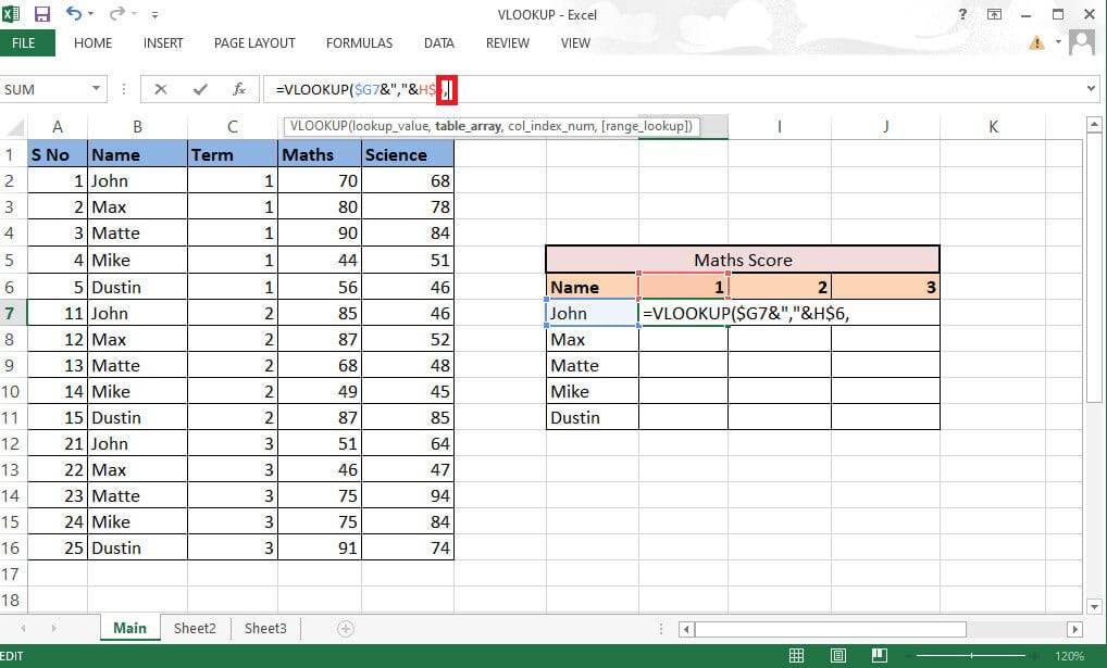
6. Here instead of table_array , use CHOOSE function.
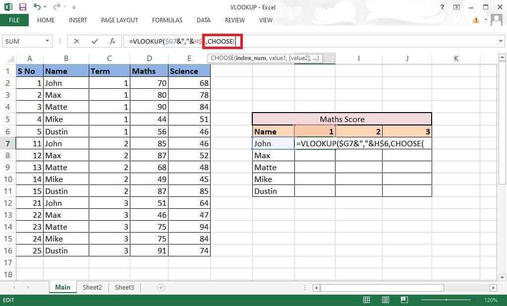
7. Write 1 In square brackets as index_num to create Collection.
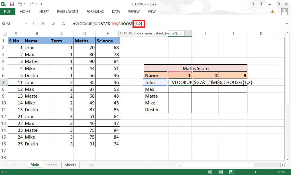
8. Write comma (،) to move to The value of the next parameter is 1..
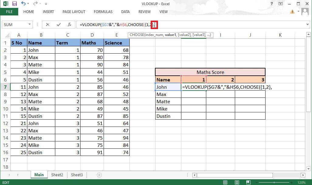
9. Select Value 1 Which will be the name column and lock the values by clicking on F4 . key.
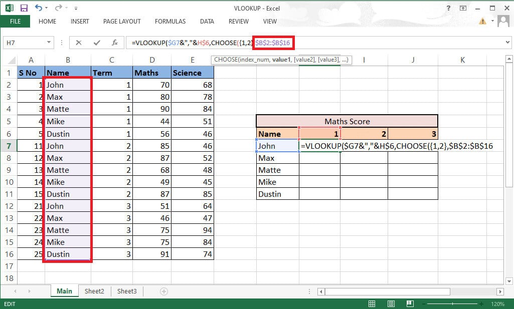
10. To integrate value1 With the next column, add Ampersand (&) with separator (,) followed by select value2 and he Term column.
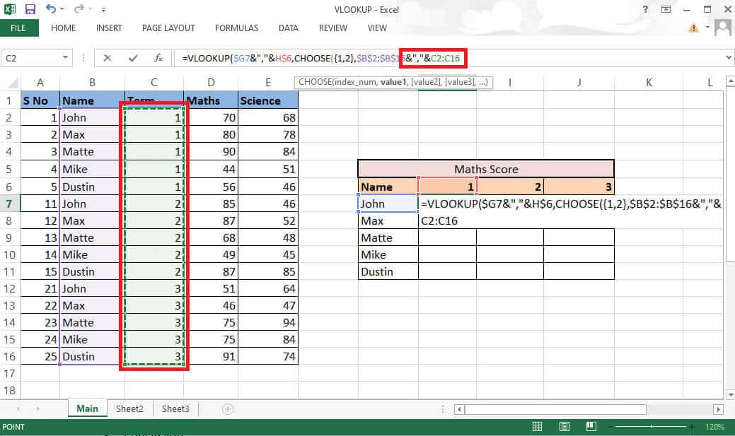
11. Lock values by pressing F4 . key And add comma (،) To move to the next parameter.

12. To add Values 2 Select the desired math column as a result, and lock the values by pressing F4 . key.
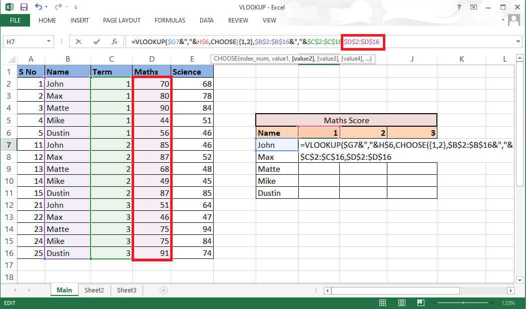
13. Close the bracket to complete the selection function. Now you have table_array Without support column.
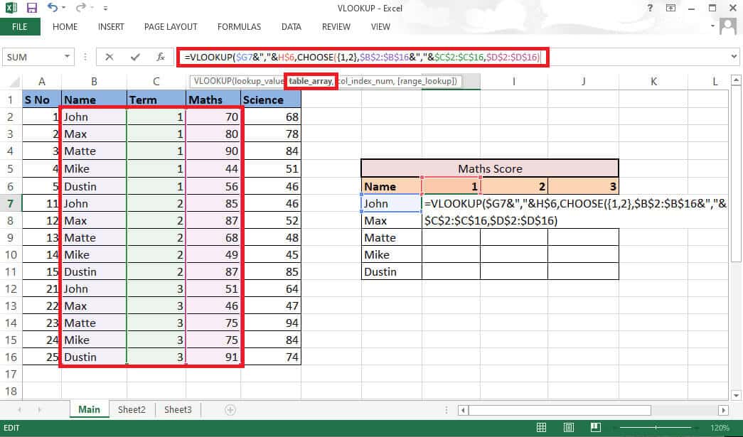
14. Write comma (,) and go to col_index_num argument , and mention 2 because math is the second column of the source column.
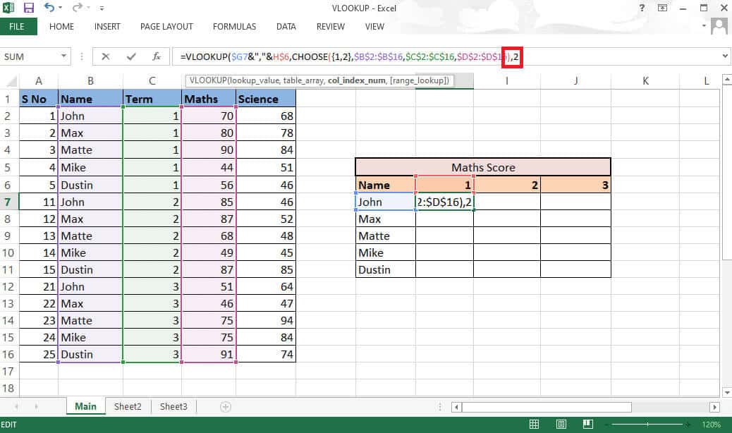
15. Add comma (،) to move to range_lookup argument and select FALSE To get the exact value.
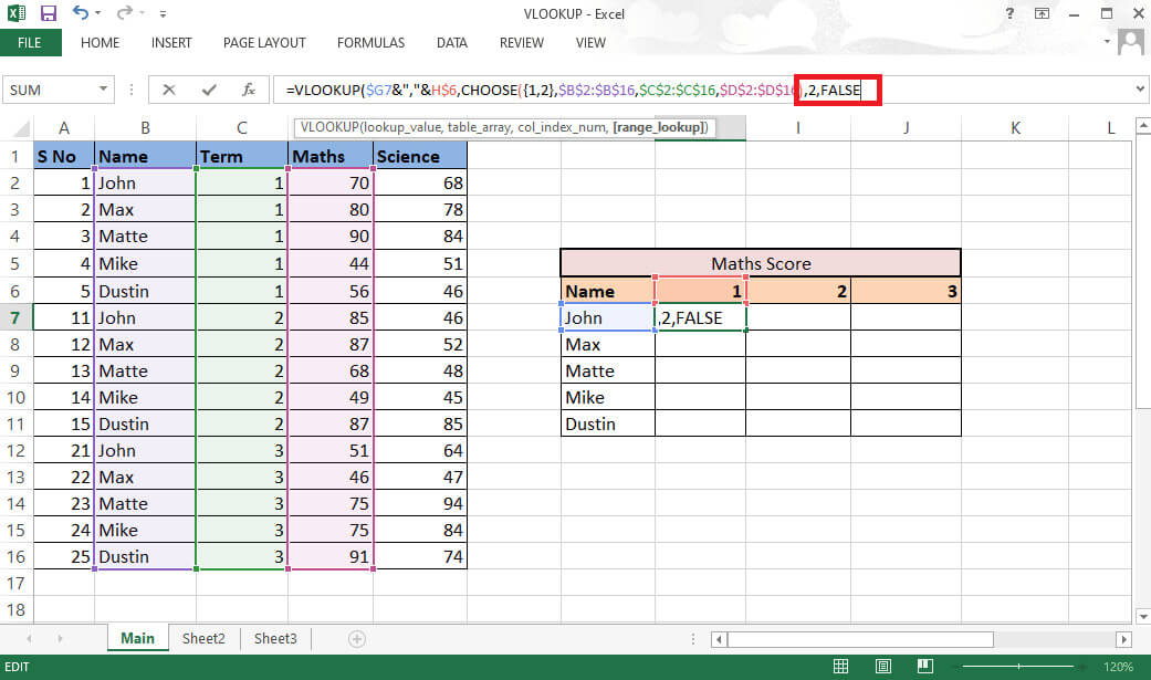
16. Close the bracket and press Ctrl + Shift + Enter To get the result.
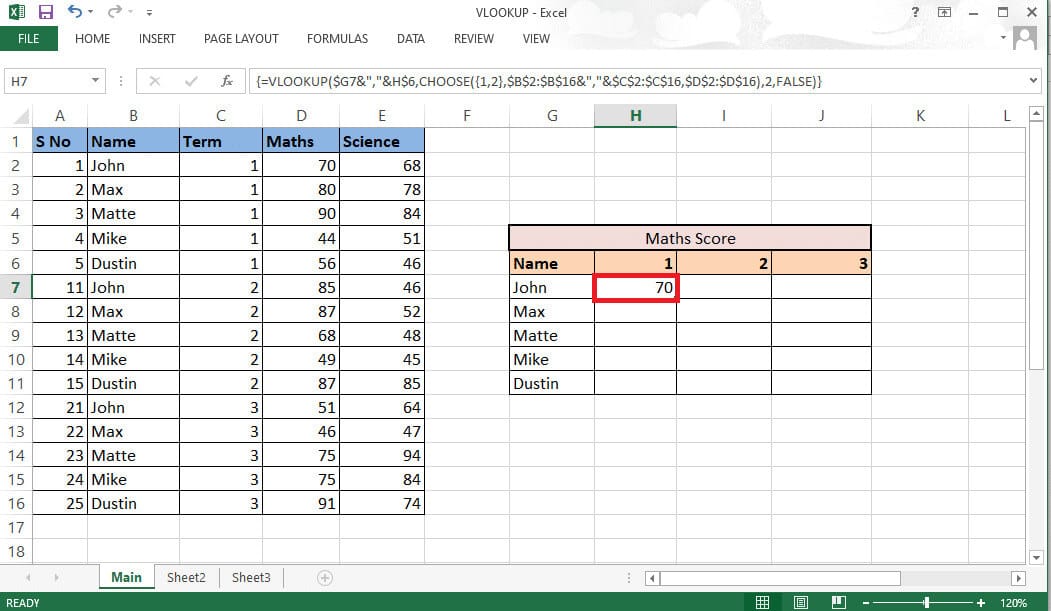
17. Pull formula Go through the table and get the full result.
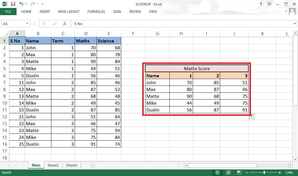
This was how to do a VLOOKUP with multiple criteria using the CHOOSE function.
Frequently asked questions (FAQs)
Q1. Why do I need to add a separator while working on groups?
answer. When we form groups without using commas, there is a possibility that we will end up with the same groups for different values. For example,
| 1 | 2 | With a break | Without a break |
| a B C | 123 | abc,123 | abc123 |
| abc1 | 23 | abc1,23 | abc123 |
Therefore, it is always recommended to use a separator to avoid this confusion.
Q2. Is it necessary to add the auxiliary column between the data?
answer. No, you can also add a helper column to the far right or left if you don't want to make any changes to the original data. However, inserting it between columns allows you to add only two columns to the table array instead of four or more. You can work as you see fit.
These were the two methods you can include when using VLOOKUP with multiple criteria. We hope this guide was helpful and that you were able to learn how to use VLOOKUP with multiple criteria and VLOOKUP with multiple criteria helper columns. Feel free to contact us with your questions and suggestions in the comments section below. Also, let us know what you'd like to know next.


