With continued use Microsoft Excel To track or Budgeting Or inventory, you may learn a lot about the available functions and their formulas. But discovering something new can be confusing or intimidating. This guide introduces a few useful functions and their formulas when you're ready to dive into new territory. Here are 5 useful advanced Excel formulas you should know.

1. Find values in your spreadsheet: XLOOKUP
When you want to look up data based on other data in a large spreadsheet, XLOOKUP is your go-to function. Unlike VLOOKUP Unlike a spreadsheet that can only search values from left to right, XLOOKUP can search values from left to right or from right to left, making it a more flexible tool.
Note: As of this writing, XLOOKUP is only available to Microsoft 365 subscribers. For other versions of Excel, check the INDEX and MATCH combination in the next section.
The function formula is:
XLOOKUP(lookup_value, lookup_range, return_range, not_found, match_mode, search_mode)
Only the first three arguments are required. A description of each argument is listed below:
- Lookup_value: The value to search for.
- Lookup_range: The range that contains the value to be searched for.
- Return_range: The range containing the value to be returned.
- Not_found: The text to return if the value is not found. “#N/A” is the default if omitted.
- Match_mode: Match type using "0" for exact match and "#N/A" for not found (default if omitted), "1" for exact match and the next smaller item if none are found, "-1" for exact match and the next larger item if none are found, or "2" for wildcard match using a question mark, asterisk, or tilde.
- Search_mode: Search mode using "1" to start from the first item (default if omitted), "-1" to start from the last item, "2" when "lookup_range" is in ascending order, or "-2" when "lookup_range" is in descending order.
For example, we are looking for sales for sector 2, so we use the following formula:
=XLOOKUP(2,A19:A24,D19:D24)
Breaking down the formula, 2 is the “lookup_value”, A19:A24 is the “lookup_range”, and D19:D24 is the “return_range” argument.
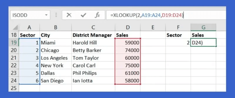
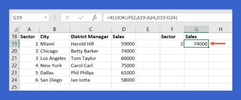
The result, 74000, is the correct corresponding value for sector 2.
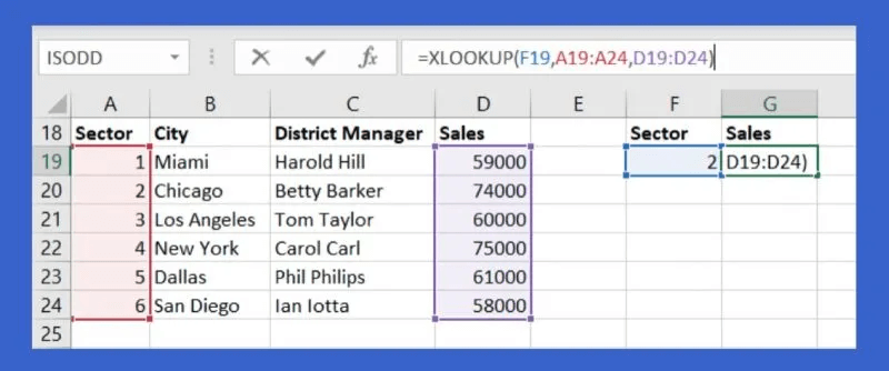
If you want something more dynamic, where you look up a value in a cell rather than a constant, and then receive the updated result whenever you change the value in that cell, see the following example:
We replace “lookup_value” 2 with cell F19:
=XLOOKUP(F19,A19:A24,D19:D24)
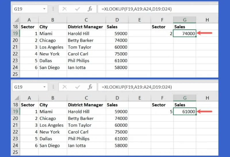
When we enter 2 in cell F19, we get the result 74000, and if we enter a different value, such as 5, we automatically get the updated result, which is 61000.
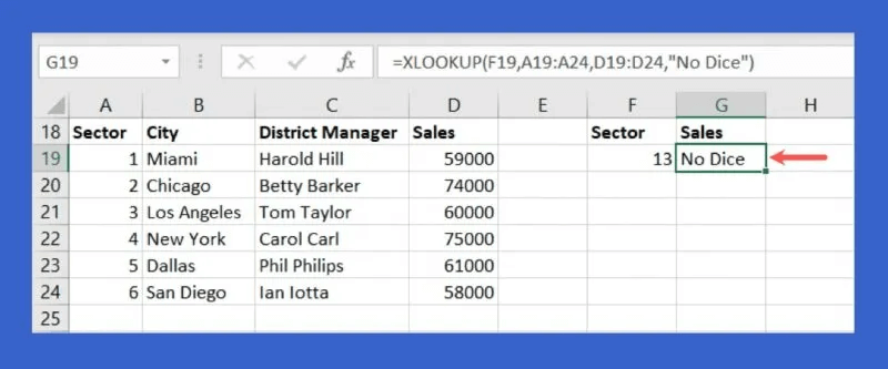
You can include the mediator. “not_found” So you don't have to look at an error message if no match is found, we add "do not reply" to the argument.
=XLOOKUP(F19,A19:A24,D19:D24,"No dice")
When a value is entered in cell F19 that does not have a match, you will see your message instead of “#NA”.
2. Find the alternative value in a sheet: INDEX and MATCH
While XLOOKUP offers a powerful way to look up values, it is currently only available to Microsoft 365 Excel subscribers. If you're using a different version of Excel, you can use INDEX and MATCH to do the same thing.
Using the INDEX function, the value in a cell is returned based on the position you enter in the formula. The INDEX formula is:
INDEX(range, row_number, column_number)
Using the MATCH function, the position of the value you enter into a formula is returned. The MATCH formula is:
MATCH(value, range, match_type)
To combine these two functions and their formulas, put the MATCH formula in the INDEX formula as the search location (“row_number” and “column_number”).
Using the same data as the XLOOKUP example above, we want to see the segment sales that we enter into cell F19. The formula is:
=INDEX(D19:D24,MATCH(F19,A19:A24))
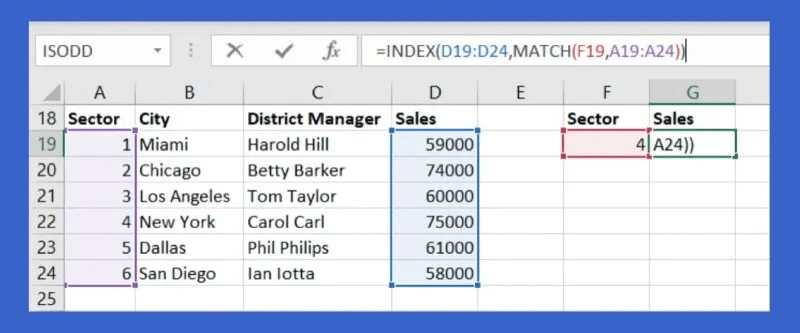
To break this formula down, we start with INDEX and its "range" argument, which is D19:D24. This is the range that contains the result we want.
The MATCH formula uses F19 as the “value” argument and A19:A24 as the “range” argument containing that value.
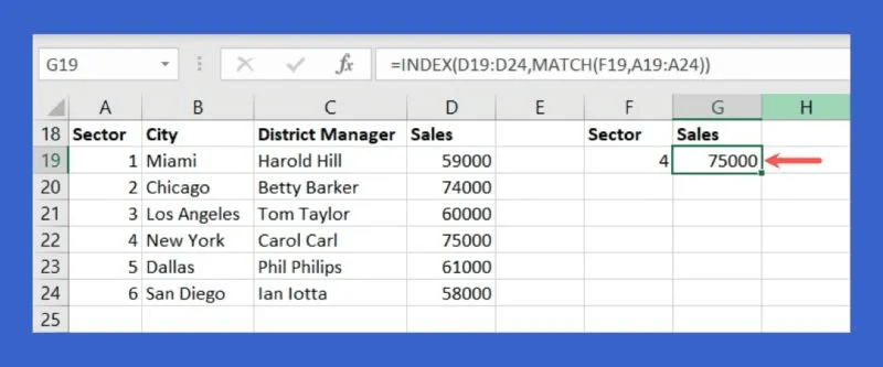
When we enter 4 in cell F19, we get the result 75000, which is correct.
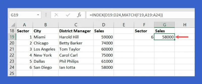
If we enter a different sector in cell F19, such as 6, the formula automatically updates to give the correct value of 58000.
3. Add or count by criteria: SUMIF, SUMIFS, COUNTIF, and COUNTIFS
The SUM and COUNT functions in Excel are designed to add numbers and count cells, but they are limited to simple arithmetic operations. Variations of these functions allow you to add or count using criteria. For example, you can only add numbers greater than 12 or count cells containing the name "Bill."
Using SUMIF and COUNTIF, you can add or count with a single condition, and using SUMIFS and COUNTIFS, you can add or count with multiple conditions. Listed below are the syntaxes for each:
SUMIF
SUMIF(range, criteria, sum_range)
COUNTIF
COUNTIF(range, condition)
SUMIFS
SUMIFS(sum_range, condition_range1, condition1, condition_range2, condition2,…)
COUNTIFS
COUNTIFS(condition_range1, condition1, condition_range2, condition2,…)
See below for an example of each function.
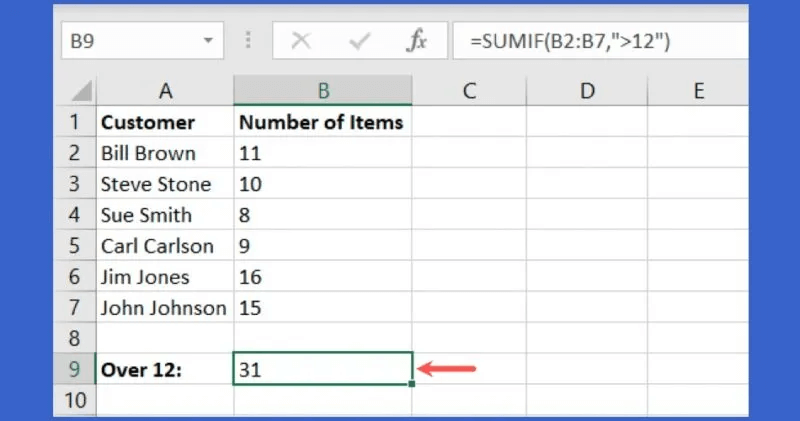
To add the numbers in our range from B2 to B7 only for numbers greater than 12, we use the SUMIF function and this formula:
=SUMIF(B2:B7,">12")
The result is 31, since the formula added 16 and 15, the only two numbers greater than 12 in the data set.
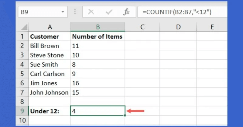
In the following example, we count cells with values less than 12 in the same range, from B2 to B7, with the following formula:
=COUNTIF(B2:B7,"<12")
The result of this formula is 4, since this is the number of cells in the range with values less than 12.
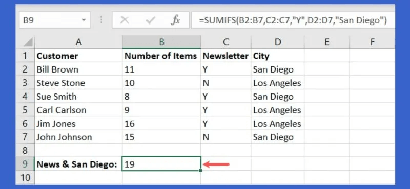
Let's take a look at SUMIFS and use two conditions. To add the numbers in cells B2 through B7 for only those who subscribed to our newsletter (Y) in cells C2 through C7 and whose city is San Diego in cells D2 through D7, we use the following formula:
=SUMIFS(B2:B7,C2:C7,"Y",D2:D7,"San Diego")
The result of this formula is 19, since there are only two clients with Y for newsletter and San Diego for city. Bill Brown has 11 items and Sue Smith has 8 items, for a total of 19 items.
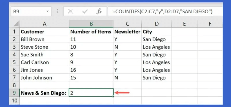
For an example using the COUNTIFS function, we count the number of cells with the same two conditions described above. We count the number of customers who signed up for the newsletter (Y) and their city is San Diego.
=COUNTIFS(C2:C7,"Y",D2:D7,"San Diego")
As expected, the score was 2 for Bill Brown and Sue Smith, the only newsletter subscription in San Diego.
4. Test data under different conditions: IFS
The IF function in Excel is a powerful tool for testing data against conditions. For example, you can use it to display a letter grade for a student's numeric score, or a "yes" if a salesperson brings in enough revenue to earn their bonus, and a "no" if they don't.
The problem with the IF function is that to test your data against multiple criteria, you must combine all of the IF statements together. To address this confusion, use the IFS function.
Similar to SUMIFS and COUNTIFS above, IFS allows you to add multiple criteria to your formula in a clear and easy-to-read way.
The syntax is IFS(test1, if_test1_true, test2, if_test2_true, …), where you can test up to 127 different criteria.
Using one of our example scenarios, we simply started by indicating the rewards. If the amount in cell B2 is higher than 20000, show "Yes". If not, show "no". The formula becomes:
=IFS(B2>20000,"Yes",B2<20000,"No")
In the first test, if the value in B2 is greater than 20000, the result if true is “yes”. In the second test, if the value in B2 is less than 20000, the result if true is "no".
Fortunately, our sales rep receives his bonus. Since his sales are 21000, the "Yeah" In the bonus column.
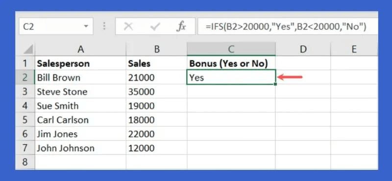
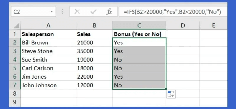
Copy the formula if you have a list like our example. Drag the fill handle in the lower-right corner of the cell to the remaining cells for the other salespeople. The formula will automatically update to include the different cell references.
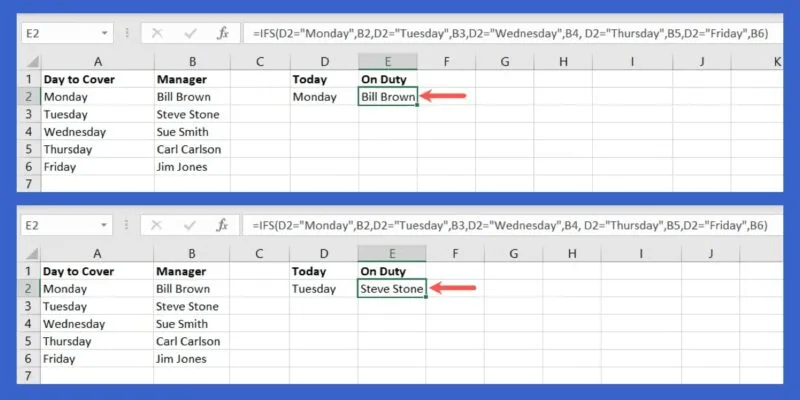
For another example from IFS, we have a list of on-duty managers for each day of the week. When the current day is displayed in cell D2, the corresponding manager's name is displayed in cell E2. The formula becomes:
=IFS(D2="Monday",B2,D2="Tuesday",B3,D2="Wednesday",B4,D2="Thursday",B5,D2="Friday",B6)
This shows that if the value in cell D2 is Monday, display the name in cell B2, if the value in cell D2 is Tuesday, display the name in cell B3, if the value in cell D2 is Wednesday, display the name in cell B3, and so on.

When you change the day of the week in cell D2, the corresponding name of the on-duty manager is displayed in cell E2.
With a little work to create the formula upfront, you can reap the benefits of some automation in your Excel sheet.
5. Filter using multiple criteria: Filter
As an Excel user, you probably know that the application comes with a built-in filtering feature. However, if you want to filter your data using a condition or even multiple criteria, you'll need to use the Filter function. This flexible function and its arguments can help you narrow down large data sets in just minutes.
The function's syntax is FILTER(range, range=criteria, if_empty), where only the first two arguments for the dataset plus the criteria and its container range are required. The third argument is useful if you want to return something in particular if the formula doesn't return zero results, such as No data Or "nothing".
It's important to understand how the FILTER function works with a single condition before adding multiple criteria. For example, you can filter the data in cells A2 through C9 by Harold Hill, which is in cells B2 through B9. The formula for this is:
=FILTER(A2:C9,B2:B9="Harold Hill")
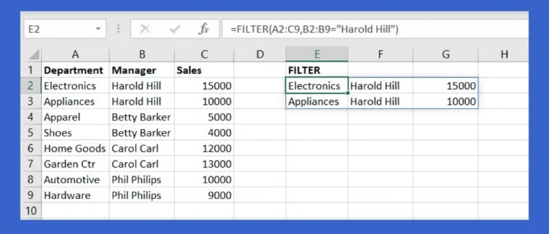
We have two results for Harold Hill. Easy, right?
Let's add more conditions to the formula. Multiple criteria are added using an asterisk (*) for AND and a plus sign (+) for OR.
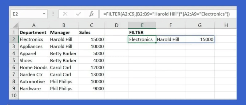
For example, we filter out both: Harold Hill و Electronics Using the following formula:
=FILTER(A2:C9,(B2:B9="Harold Hill")*(A2:A9="Electronics"))
To split the formula, A2:C9 is the data set, B2:B9 = “Harold Hill” It is the first condition, and the asterisk represents AND, and A2: A9 = “Electronics” It is the second condition.
We got one result with our filter, where the formula should match both conditions, Harold Hill and Electronics.
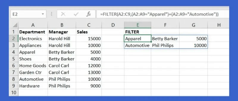
In another example, you can filter by clothes or cars:
=FILTER(A2:C9,(A2:A9="Apparel")+(A2:A9="Automotive"))
By dividing this formula, A2:C9 is the data set, A2:A9 = “Apparel” It is the first condition, and the plus sign represents OR, and A2:A9 = “Automotive” It is the second condition.
This time, we get two results, since the formula should match either condition – not both.
Frequently Asked Questions
Q1: How can I find the formula structure of a function directly in Excel?
The answer: Excel provides a built-in tool to find the function you need. Using it, you can see the syntax of that function's formula.
Select an empty cell, go to the Formulas tab, and choose Insert Function on the left side of the ribbon. Type the function in the search box at the top and click Go. When you see the function you want, select it to see its description and syntax at the bottom of the box.
Q2: How can I correct a formula that is not working properly?
The answer: Select the formula you're struggling with and go to the Formulas tab. Select Evaluate Formula in the Formula Audit section of the ribbon.
You'll see your formula in the Evaluate Formula window, with a portion of it underlined. Click Evaluate to see the calculation of the underlined portion. Continue this process to step through each portion of the formula to the result. This lets you see how the formula is being processed and where errors may have occurred.
Q3: How can I find out why I received a formula error?
The answer: When you see an error in a formula you've created, you can do two things to get more information. First, click the error button that appears next to the cell, and then select "Help on this error" to get more details from Microsoft in the sidebar that appears.
Alternatively, select "Show Calculation Steps" to open the Formula Evaluation window shown above. You'll see the result of the calculation and the process involved, which should help identify the cause of the error.


