How to Find and Remove Duplicates in Excel

Duplicate values in Excel can be annoying, but fortunately, there are several ways to find and remove them. We recommend backing up your Excel worksheet before removing duplicates. Let's take a look at how to find, count, and remove duplicate values in Excel.

1. Use the Remove Duplicates button.

Excel comes with a native button to remove duplicate values.

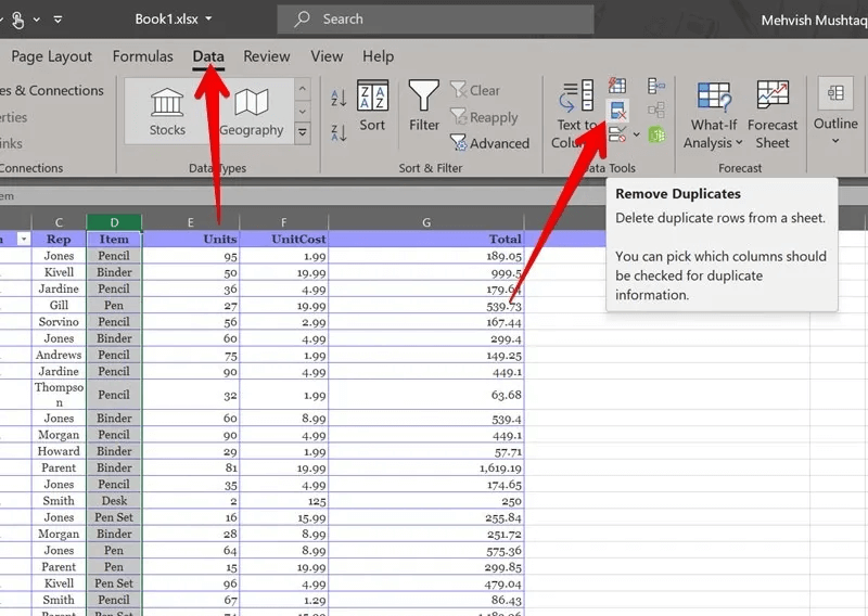
1. Locate column in which you want to remove duplicates.
2. Go to the tab Data and click the . button “Remove duplicates.”

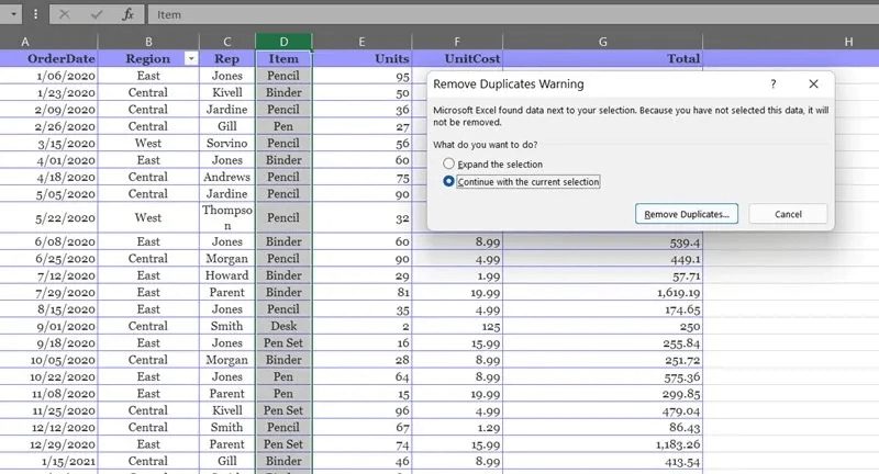
3. A warning box will appear. "Repetitions" , allowing you to customize your selection.
4. Select the option "tracking With current selection” To remove duplicates from the currently selected dataset.
5. To include more columns in the list, select Expand selection.
6. Press the . button “Remove duplicates” either way.

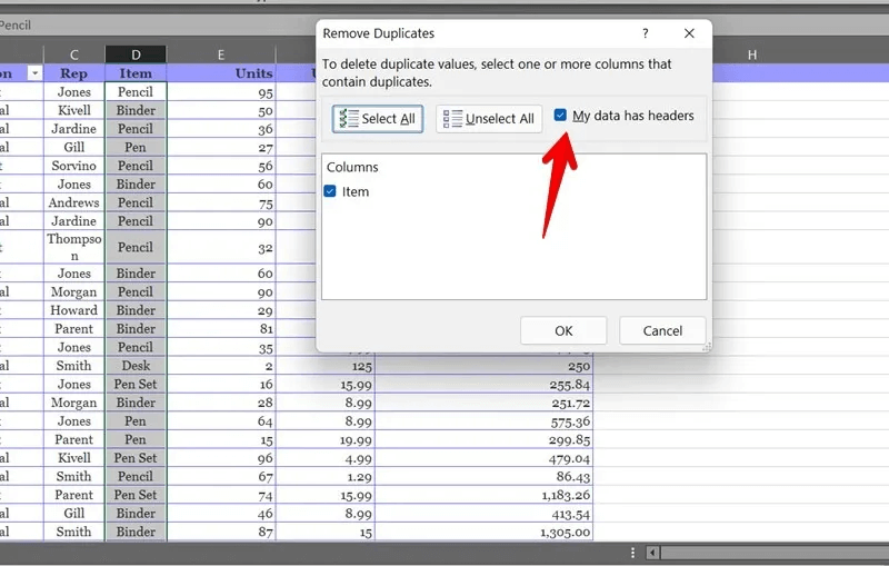
7. Keep the box checked next to the columns that contain duplicates and deselect that you want to keep them.
8. Make sure the box next to My data contains headers.This will keep the first sets of data for duplicate values while removing their subsequent entries.

9. Click the button "OK". Excel will remove all duplicate values and provide a summary of the number of duplicate and unique values found.

2. Find duplicate data using conditional formatting

This duplicate removal method is based on conditional formatting and will help you find duplicate values without deleting them.

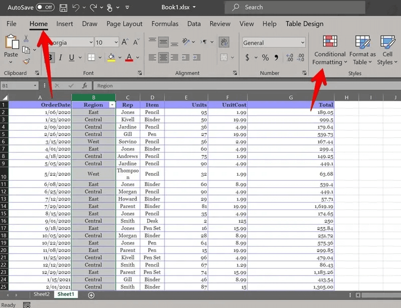
1. In an Excel sheet, select the data that contains duplicates. This can be a column or the entire table.
2. Go to the tab Home page and click Police coordinationDuplicate values will be highlighted.

3. Choose “Cell base recognition” followed by “Duplicate values”.

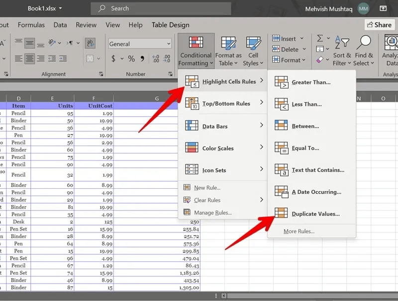
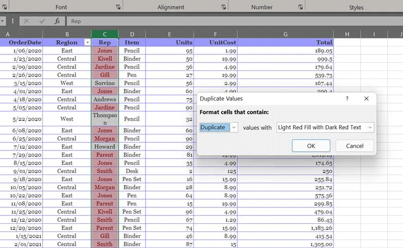
4. The pop-up window will appear. “duplicate values” , allowing you to change the color of duplicate values.
5. Click the drop-down box. "repetition" and select "unique" If you want to see unique values instead.
6. Click "OK".

3. Remove duplicates using a conditional filter

With duplicates highlighted, you can either use filters to remove them or use the method described above.

1. To activate the filtering process, go to Home tab → Sort & Filter → Filter.

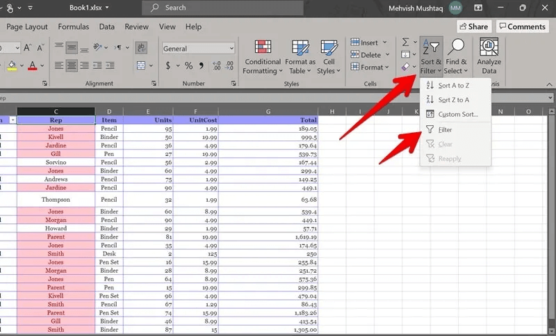
2. A drop-down box will appear next to the column headings in your data. Click the drop-down box in the column where you want to filter for duplicates.
3. Select Filter by color From the menu, choose the color of the unique values to keep in your worksheet and remove duplicates.

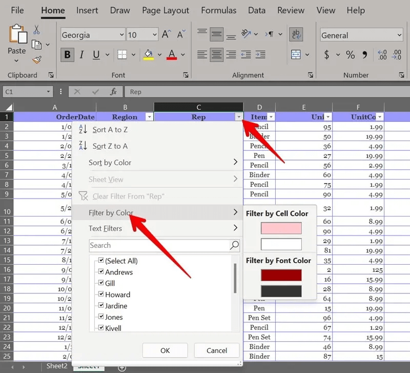
4. Your sheet will now display only unique values. Be careful because this method removes all duplicate values, including the first one.

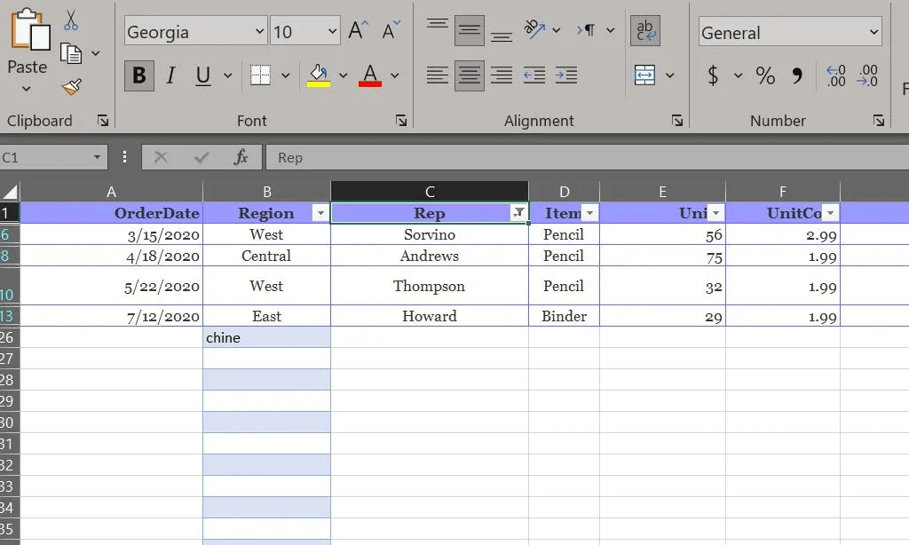
To copy unique values, select the data set and use Alt+ ; Keyboard shortcut to select only visible rows, then use the shortcut Ctrl + C To copy and paste visible rows wherever needed.

4. Find duplicate values using a formula

Duplicates in a column can also be found using Excel formulas. The basic formula for detecting duplicate entries is: =COUNTIF(Range, Criteria) >1  =COUNTIF(range, criteria)>1 , where the range can be the entire column or a subset of rows.

Create a new column and enter one of the commands below in the new column.

• Use the formula =COUNTIF(D:D, D2) >1  For a full column, where D It is the name of the column and D2 It is the top cell.
• For selected rows, use the formula =COUNTIF($D$2:$D$10, $D2) >1, where the first group represents the selected rows, and D2 is the top cell. Please note that the range must be preceded by a dollar sign ($), otherwise the cell reference will change when you drag the formula.

Drag the fill handle to use the command in other rows. The formula will display "right" For duplicate values and "Error" For unique values.

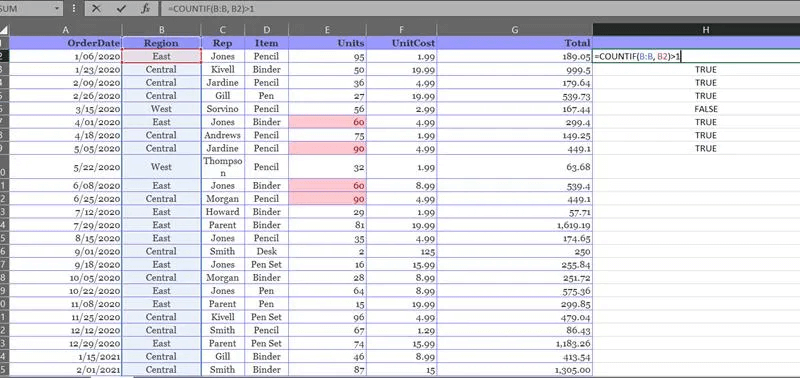
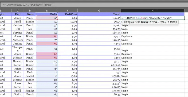
If you want to display text other than True Or False You must attach the COUNTIF formula to the function. IF. So the formula will become =IF(COUNTIF($D$2:$D$10, $D2) > 1, "Duplicate”, “Single”).

If you want unique values to show in a blank cell, use the formula  =IF(COUNTIF($D$2:$D$10, $D2) > 1, “Duplicate”, “”).

5. Count the number of repetitions using the formula

You can use the above formula without the text.> 1 To count the number of occurrences in a column. The two formulas will become =COUNTIF($D$2:$D$10, $D2)  و  =COUNTIF(D:D, D2)Enter in the new column to display the number of times each item appears in the data.

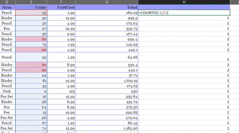
6. Remove duplicate values using a formula

Once you find duplicate values or a duplicate count, use the filter method to remove the duplicates and keep the unique values.

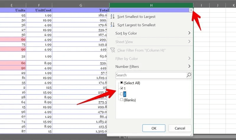
1. Go to Home tab -> Sort & Filter -> Filter To enable the drop-down filter list box in the column header.
2. Click it and keep the box checked next to the value you want to keep. It should be "Unique" How to find duplicates and "1" To count duplicates. Doing so will hide duplicate values and display unique values.
3. Select visible rows using Alt + ; shortcut.

7. Remove duplicate data using advanced filters

1. Go to the tab Data and click "Advanced Options".

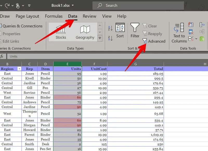
2. A pop-up window will open. "Advanced candidate."
3. Select the option “List filter, in the same place” If you want to hide duplicates in the same data set, you can manually copy the unique values and paste them later to a different location in the same or a different sheet.
4. With this option selected, select the column list. It will automatically appear in the field. List scopeLeave. "range of standards" Empty.
5. Check the box next to Unique records only And press "OK".

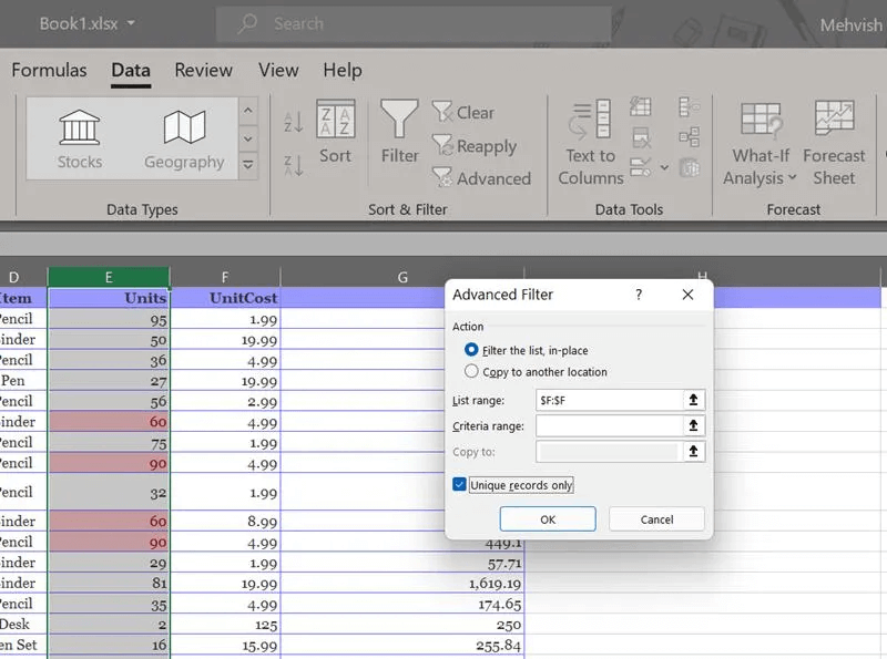
6. This will display unique values in your data. Use Alt + ; shortcut To select rows that are visible only if you want to perform any action on them.
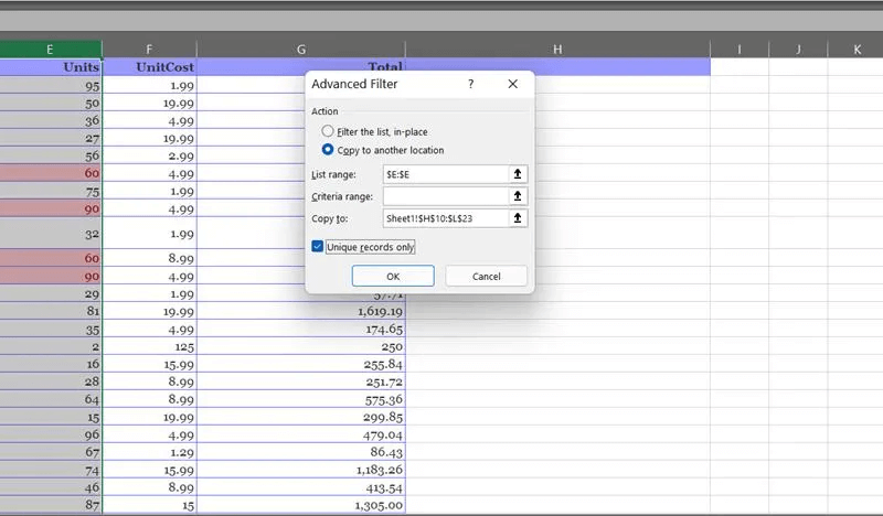
7. Conversely, specify “Copy to another location” If you want Excel to automatically copy the unique values to a different location in the same sheet.
8. Select List scope First, you can leave "range of standards" Empty.
9. Click once on a field. Copy to Select the rows on the sheet where you want to copy the unique data.
10. Make sure the box next to Unique records only.

8. Remove duplicates in Excel using Power Query

Power Query also helps to remove duplicate values in Excel as shown below.

1. Select the values where you want to remove duplicates.
2. Go to the tab Data and click From table/range.

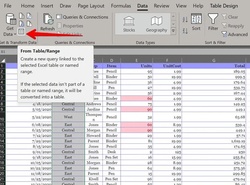
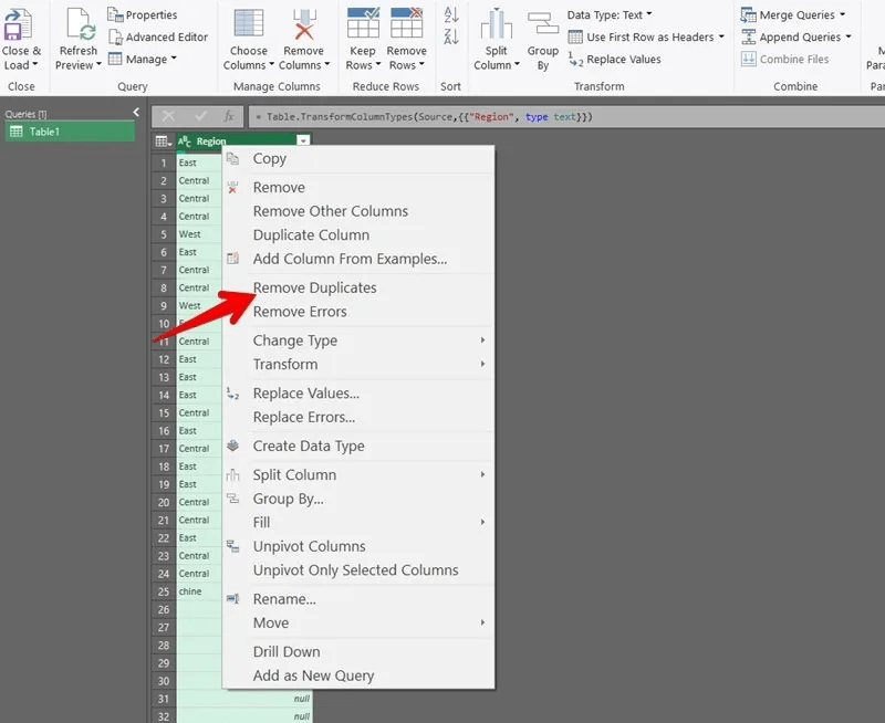
3. The editor will open. Power QuerySelect the columns and right-click on the column header. Choose “Remove duplicates” from the list.

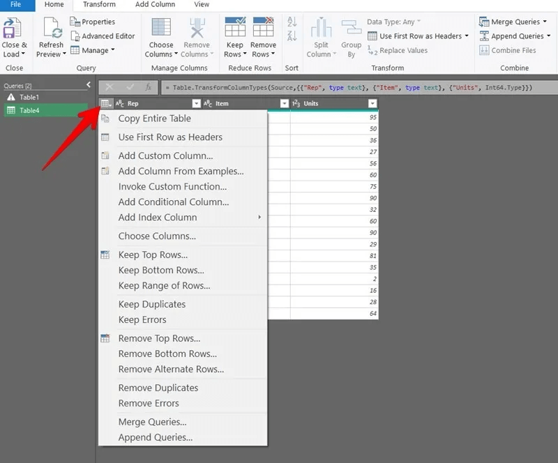
4. If you want to remove duplicates from the entire table, click the button. "table" In the upper left corner and choose “Remove duplicates.” Instead, select Keep duplicates To display only duplicate entries and remove the rest.

Click Close and load At the top to open the table in the same sheet.

9. Using pivot tables

you can use Pivot tables To display only unique values in your data, thus removing duplicate entries.

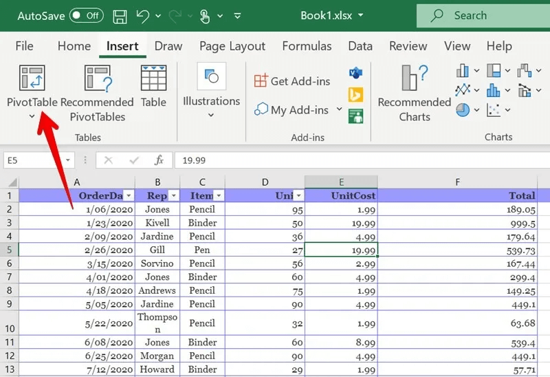
1. Start creating a pivot table by selecting a cell within your data.
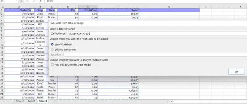
2. Go to Insert → Pivot Table.Select From table/range.

3. It will be opened PivotTables From the table or Pop-up range.
4. Select the table or range in which you want to hide duplicate values, so that they automatically appear in a field. Table/Range
5. Determine whether to place PivotTables In the same worksheet or in a new worksheet.
6. Click “Okay.”

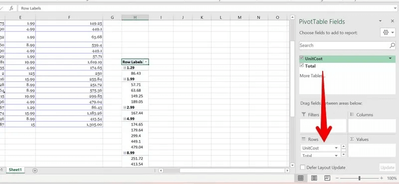
7. You will be welcomed by the sidebar. PivotTable fieldsDrag the columns where you can extract unique values to a section. "rows"

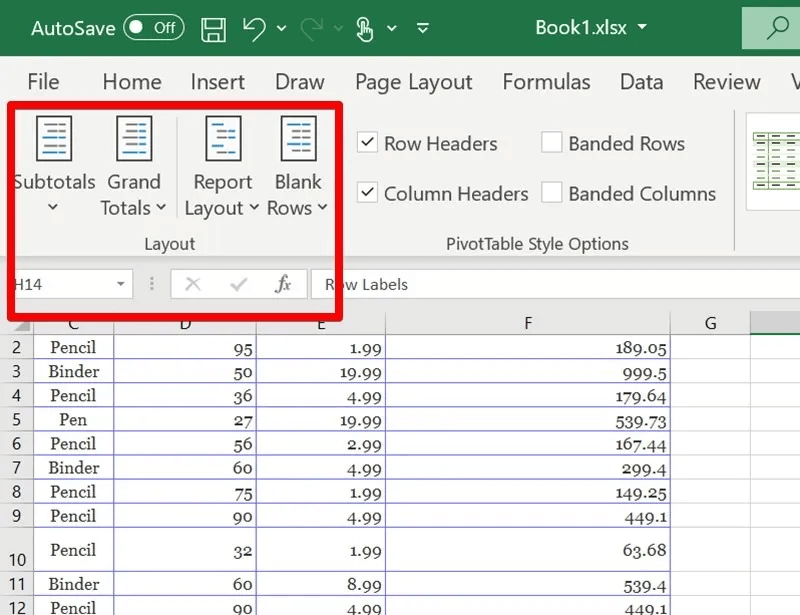
You'll need to format your PivotTable to display it in tabular form. To do this, go to the Data tab and perform the following steps:

1. Click “Report Layout → Show” in table form.
2. Go to Subtotals → Don't show subtotals.
3. Click “Report Layout → Repeat All Item Labels”.
4. Under Grand Totals, select Off for Rows and Columns.

You will get a pivot table with unique values in tabular form.

Excel

Read on to find out. How to analyze data in Microsoft Excel If your worksheet contains important data, learn how to Password protect an Excel workbook.