When you import data or text into Microsoft Excel, it appears in a different format. The format in which the text or data appears depends on the source of the data or text. For example, customer names or employee addresses. By default, this data appears as a continuous string in a single cell. Here are the top 3 ways to split text or data in Microsoft Excel.

If you encounter such a situation, Microsoft Excel offers various features you can use to segment such data. In this post, we cover some fixes you can try.
Use Flash Fill
Excel's Flash Fill feature lets you add an example of how you want to split data. Here's how:
Step 1: Run the Excel file with the relevant data.

Step 2: In an Excel worksheet, provide an example of how you would like to split the data or text in the first cell.
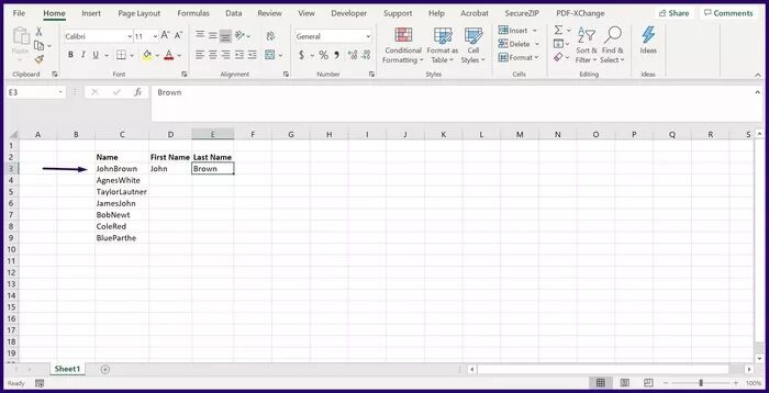
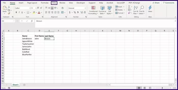
Step 3: Click the next cell you want to fill, and on the ribbon, click Data.
Step 4: In the Data Tools group, click Flash Fill and this should split the data into the remaining cells in the selected row.
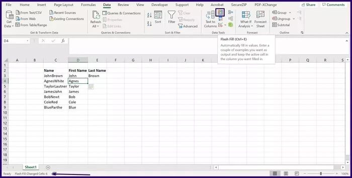
Flash Fill has some limitations. For example, it doesn't correctly extract numbers with decimals. It only enters numbers after the decimal point. As such, you may still need to manually verify that your data has been accurately segmented.
Using the selector function
A delimiter function is a string of characters used to define boundaries between independent and separate regions in data streams. You can also use it to separate mathematical expressions or plain text in Excel. Some examples of delimiter functions in Excel include commas, dashes, spaces, hyphens, and colons.
Here's how to use the selector function:
Step 1: Run the Excel file with the relevant data.
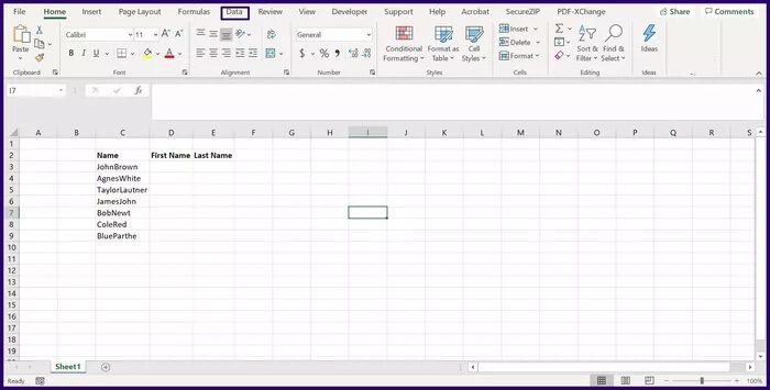
Step 2: Select the list of columns you want to split and click Data in the Excel ribbon.
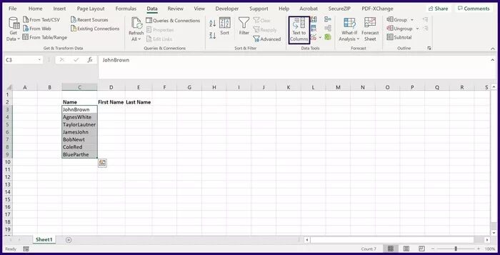
Step 3: Click Text to Columns, and this should launch a dialog box called the Convert Text to Columns Wizard.
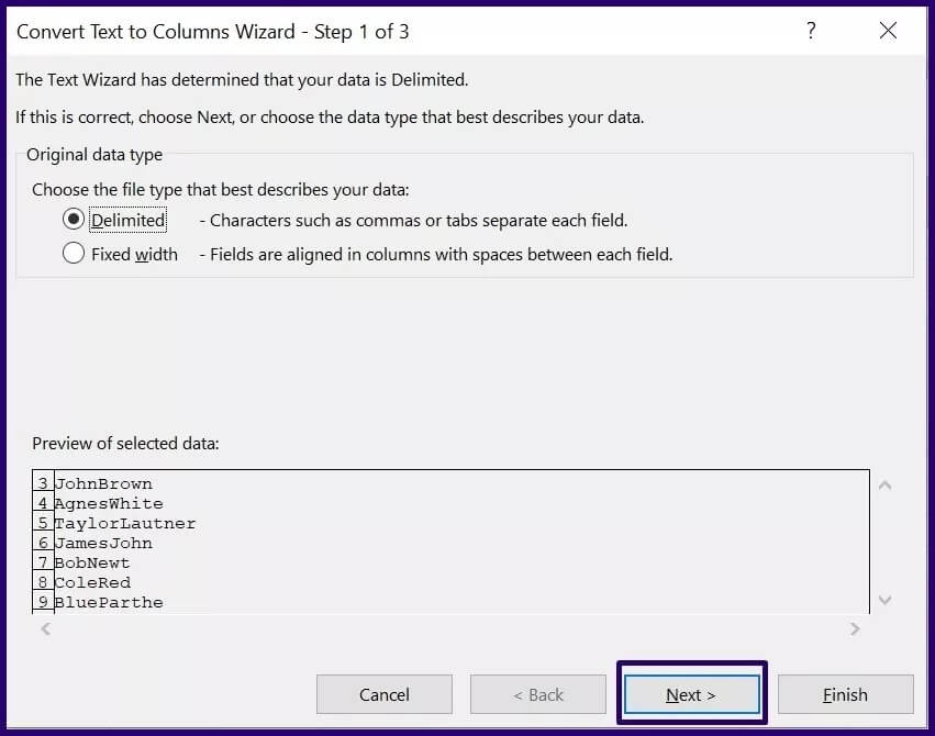
Step 4: Select the specific job from the two available options and click Next.
Step 5: On the next page of the Convert Text to Columns wizard, select the delimiter you need to split your data (for example, Tab, Space, etc.) and click Next. If you want to use a custom delimiter, click Other and provide the delimiter in the next box.
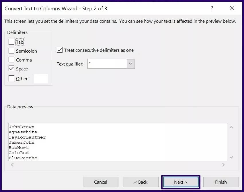
Step 6: On the last page, select the partitioned data format and preferred destination.
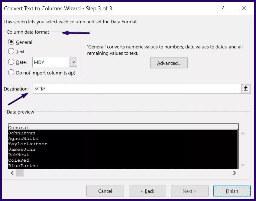
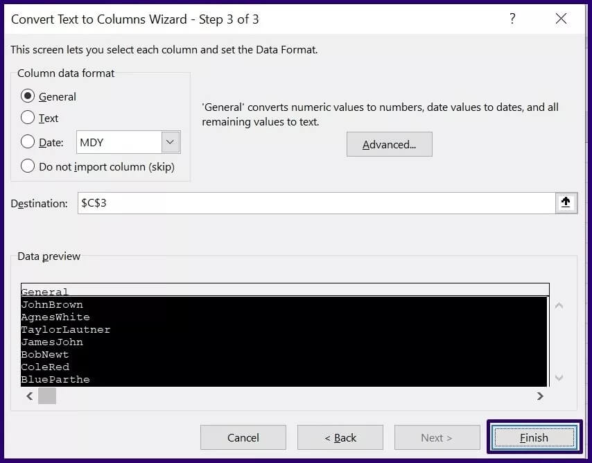
Step 7: Click Finish and the data should be split into multiple cells using the specified delimiter.
Using Power Query
Power Query allows Excel users to manipulate columns into sections using delimiters. The steps below will show you how to use this method to segment text or data:
Step 1: Start Excel.

Step 2: Go to the Excel ribbon and click on Data.

Step 3: Click Get Data.
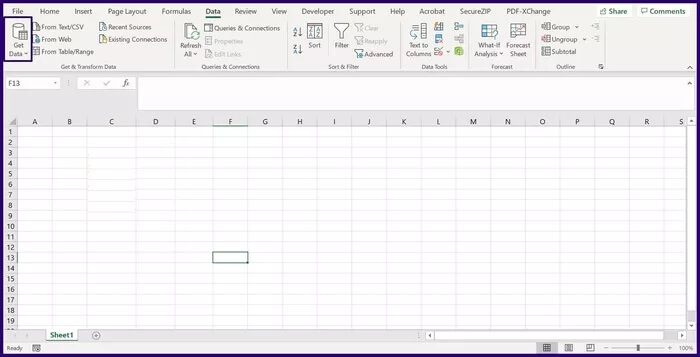
Step 4: Select From File from the first dropdown and From Workbook from the second dropdown and this should launch File Explorer.
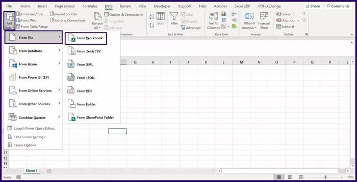
Step 5: Click the Excel workbook with the relevant data and click Import.
Step 6: You should see a navigation pop-up window displaying the worksheets in your workbook. Select the worksheet with the relevant data to see a preview.
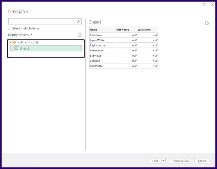
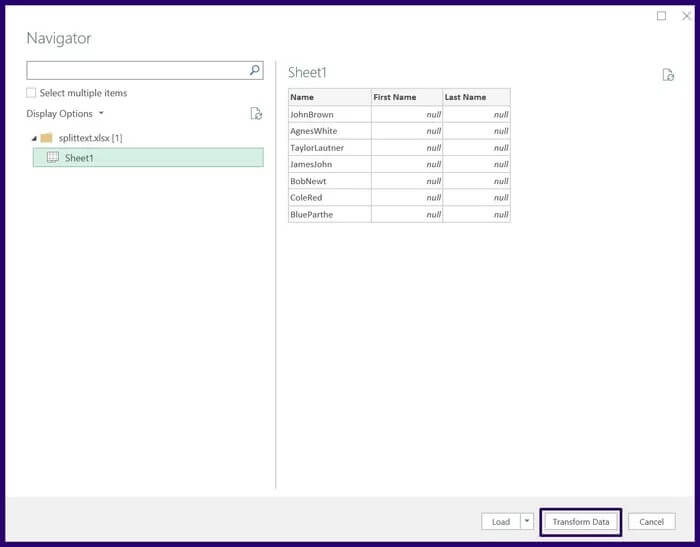
Step 7: Select Transform to show the Power Query Editor.
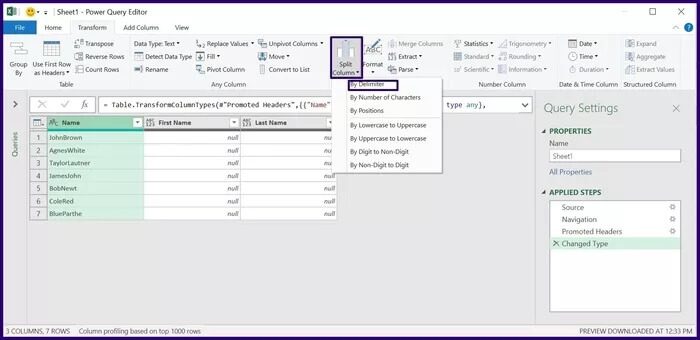
Step 8: Under Text Group, select Split Column, and from the drop-down menu, select By Delimiter.
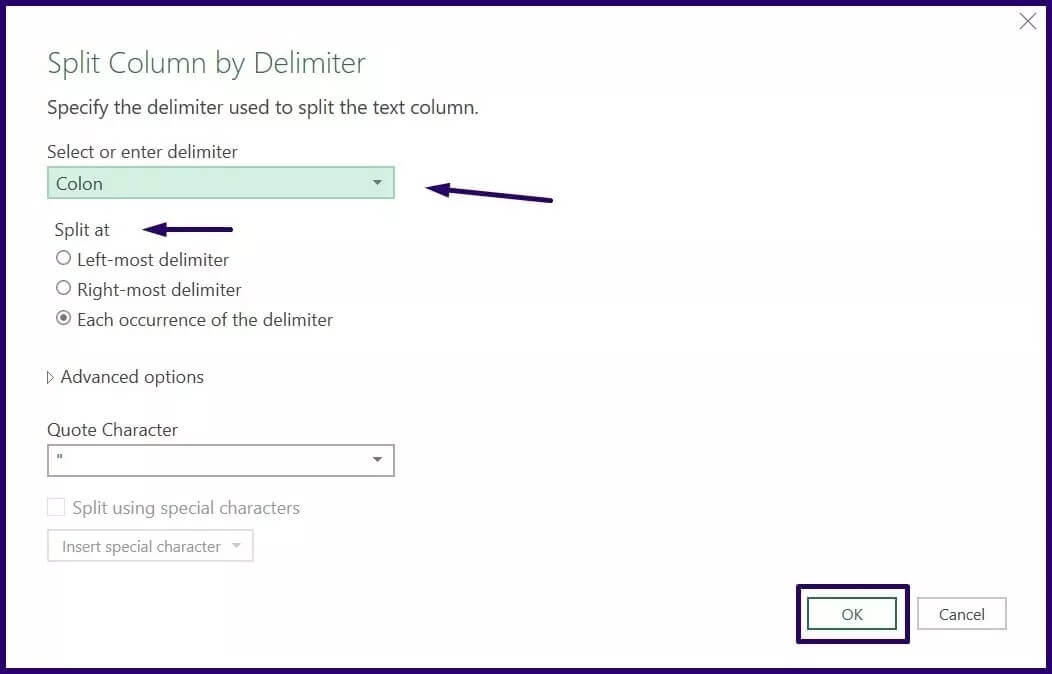
Step 9: In the Split Column by Delimiter dialog box, select the Delimiter type and the split point, and then select OK.
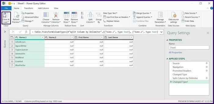
Step 10: On the Home tab, click Close and you'll see a new worksheet displaying the split data.
Import data into Excel
Splitting text or data in Microsoft Excel is extremely important if you find yourself having to manually clean up your data to fit your preferred analysis format. Aside from the best presentation, you also want your data to make sense and be usable elsewhere.
Using any of the above methods should help you split text or data in Microsoft Excel, thus reducing the time spent cleaning data. Another way to save time and effort in cleaning data is by Import data correctly into Excel.


